import numpy as np
import matplotlib.pyplot as plt

from scipy import ndimage, signal, optimize, linalg
from sklearn.model_selection import train_test_split
from sklearn.metrics import accuracy_score, confusion_matrix

np.set_printoptions(precision=4, suppress=True)Python Reference for Computer Vision Labs
NumPy, Matplotlib, SciPy, scikit-learn, and Colab tools for The Mathematics of Modern Computer Vision
Python Reference for the Computer Vision Labs
This page is a practical reference for the computer labs in The Mathematics of Modern Computer Vision. It is not a replacement for the mathematical chapters. Instead, it explains the Python tools students will repeatedly use when implementing the ideas from the book.
The guiding principle is simple:
In computer vision, an image is both a mathematical object and a numerical array.
A grayscale image is often represented as a matrix
\[ I \in \mathbb{R}^{H \times W}, \]
and a color image is often represented as a three-dimensional array
\[ I \in \mathbb{R}^{H \times W \times C}, \]
where \(H\) is height, \(W\) is width, and \(C\) is the number of channels. Most Python code in the labs is about carefully translating mathematical operations on images, vectors, matrices, functions, probabilities, and optimization problems into reliable array computations.
1. Recommended Colab Setup
Each notebook can be opened in Google Colab from the repository:
https://github.com/wanghemath/Book-MathCVA typical lab begins with imports like the following.
For reproducible experiments, set a random seed.
rng = np.random.default_rng(2026)The labs mostly use packages already available in Google Colab:
numpyfor arrays, vectors, matrices, random numbers, and linear algebra.matplotlibfor plotting images, curves, histograms, and diagnostics.scipyfor filtering, optimization, distance transforms, morphology, and numerical routines.scikit-learnfor classical machine learning tools, metrics, PCA, clustering, and train/test splits.tensorflowis optional in selected modern AI labs.
2. Images as Arrays
2.1 Grayscale images
A grayscale image is usually a two-dimensional array.
H, W = 80, 120
Y, X = np.mgrid[0:H, 0:W]
image = np.exp(-((X - 60)**2 + (Y - 40)**2) / (2 * 18**2))

print(image.shape)
print(image.min(), image.max())
(80, 120)
0.0003272810231830983 1.0The first index is the row coordinate and the second index is the column coordinate.
image[row, column]Mathematically, we often write a point as \((x,y)\), where \(x\) is horizontal and \(y\) is vertical. In NumPy, this corresponds to
image[y, x]This distinction is one of the most common sources of bugs in computer vision.
2.2 Color images
A color image is usually a three-dimensional array.
rgb = np.zeros((H, W, 3))
rgb[..., 0] = X / (W - 1)       # red channel
rgb[..., 1] = Y / (H - 1)       # green channel
rgb[..., 2] = image             # blue channel

print(rgb.shape)
(80, 120, 3)The usual channel order in Matplotlib and most deep learning code is RGB:
image[row, column, channel]Some libraries, especially OpenCV, use BGR order. When moving between libraries, always check the channel convention.
3. Displaying Images
3.1 Basic image display
plt.figure(figsize=(5, 3))
plt.imshow(image, cmap="gray")
plt.title("Grayscale image")
plt.axis("off")
plt.show()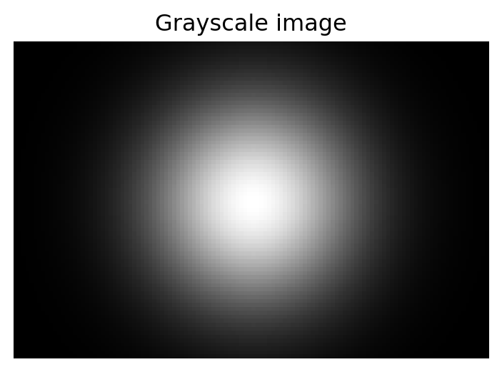
For grayscale images, use cmap="gray". For color images, do not pass a colormap.
plt.figure(figsize=(5, 3))
plt.imshow(rgb)
plt.title("RGB image")
plt.axis("off")
plt.show()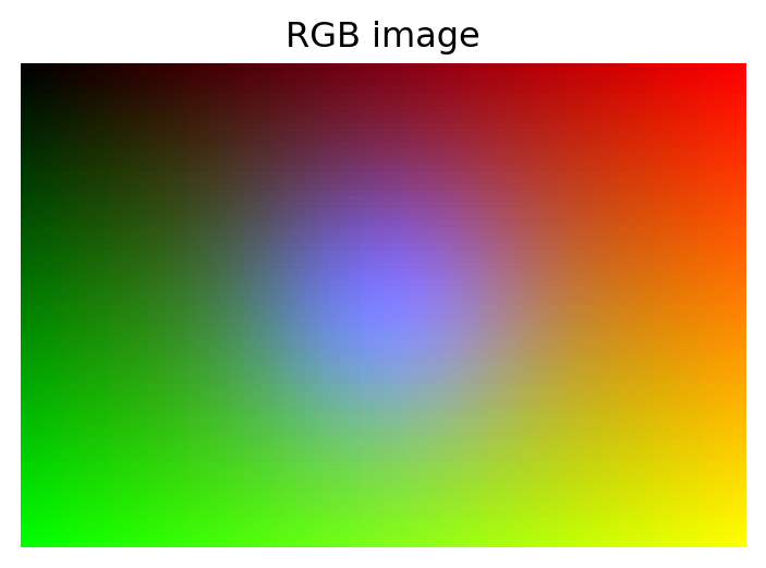
3.2 Fixing intensity ranges
When comparing images, use the same display scale.
noisy = image + 0.15 * rng.normal(size=image.shape)
blurred = ndimage.gaussian_filter(noisy, sigma=2.0)

plt.figure(figsize=(9, 3))

plt.subplot(1, 3, 1)
plt.imshow(image, cmap="gray", vmin=0, vmax=1)
plt.title("Original")
plt.axis("off")

plt.subplot(1, 3, 2)
plt.imshow(noisy, cmap="gray", vmin=0, vmax=1)
plt.title("Noisy")
plt.axis("off")

plt.subplot(1, 3, 3)
plt.imshow(blurred, cmap="gray", vmin=0, vmax=1)
plt.title("Blurred")
plt.axis("off")

plt.show()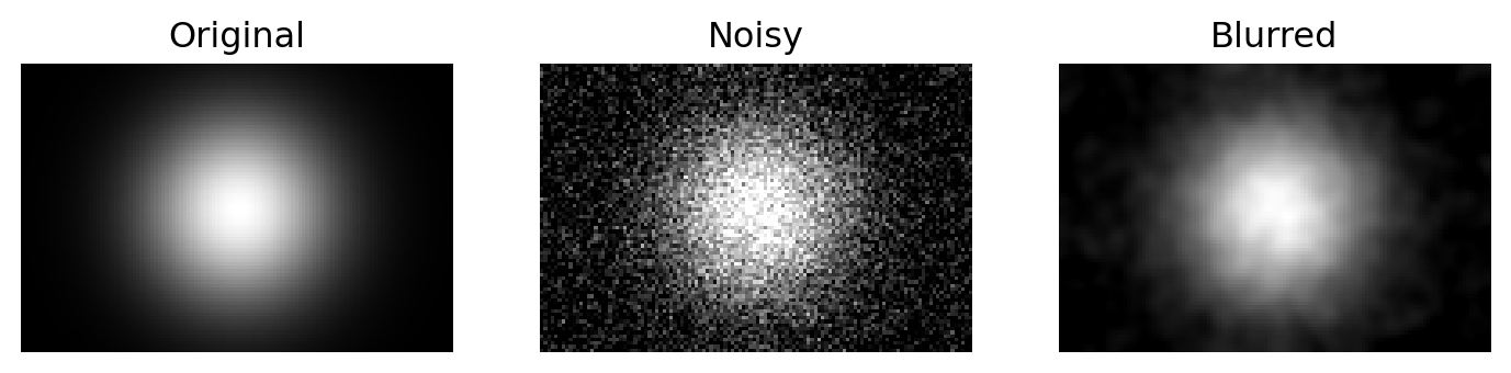
If vmin and vmax are omitted, Matplotlib rescales each image separately. That can make two different images look more similar than they really are.
4. Array Shape, Indexing, and Slicing
4.1 Shape conventions
Common image shapes:
| Object | Shape | Meaning |
|---|---|---|
| Grayscale image | (H, W) |
height by width |
| RGB image | (H, W, 3) |
height by width by channels |
| Batch of grayscale images | (N, H, W) |
number by height by width |
| Batch of RGB images | (N, H, W, 3) |
number by height by width by channels |
| Flattened image | (H * W,) |
vectorized image |
| Data matrix | (N, d) |
samples by features |
4.2 Slicing patches
patch = image[25:55, 45:75]

plt.figure(figsize=(3, 3))
plt.imshow(patch, cmap="gray", vmin=0, vmax=1)
plt.title("Image patch")
plt.axis("off")
plt.show()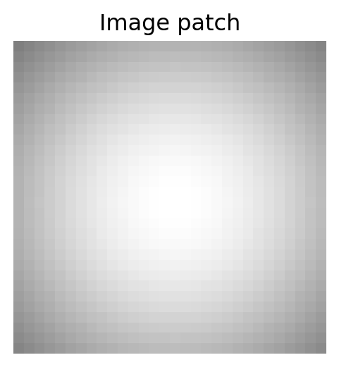
The slice image[25:55, 45:75] means rows 25 through 54 and columns 45 through 74.
4.3 Boolean masks
Boolean masks are useful for segmentation.
mask = image > 0.5

plt.figure(figsize=(5, 3))
plt.imshow(mask, cmap="gray")
plt.title("Binary mask")
plt.axis("off")
plt.show()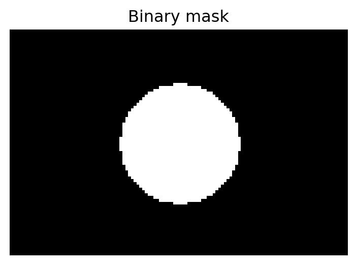
A mask can be used to compute statistics inside a region.
mean_inside = image[mask].mean()
mean_outside = image[~mask].mean()
print(mean_inside, mean_outside)
0.721019382210922 0.117465632478391955. Data Types and Normalization
Images may be stored as integers or floats.
image_uint8 = (255 * image).astype(np.uint8)
image_float = image_uint8.astype(float) / 255.0

print(image_uint8.dtype, image_uint8.min(), image_uint8.max())
print(image_float.dtype, image_float.min(), image_float.max())
uint8 0 255
float64 0.0 1.0Important conventions:
uint8images usually use values from 0 to 255.- Floating point images usually use values from 0 to 1.
- Many machine learning models expect floating point arrays.
- Before optimization or learning, normalize features when scales are very different.
A safe normalization helper is:
def normalize01(a, eps=1e-12):
    a = np.asarray(a, dtype=float)
    return (a - a.min()) / (a.max() - a.min() + eps)
6. Coordinates, Grids, and Functions
6.1 Coordinate grids
Use np.mgrid or np.meshgrid to create coordinate arrays.
H, W = 100, 140
Y, X = np.mgrid[0:H, 0:W]

circle = ((X - 70)**2 + (Y - 50)**2) <= 25**2
The arrays X and Y have the same shape as the image. They store the coordinate at each pixel.
6.2 Continuous functions sampled on a grid
x = np.linspace(-2, 2, W)
y = np.linspace(-1.5, 1.5, H)
Xc, Yc = np.meshgrid(x, y)

f = np.sin(4 * Xc) * np.cos(3 * Yc)

plt.figure(figsize=(5, 3))
plt.imshow(f, cmap="gray", extent=[x.min(), x.max(), y.max(), y.min()])
plt.title("Sampled continuous function")
plt.colorbar()
plt.show()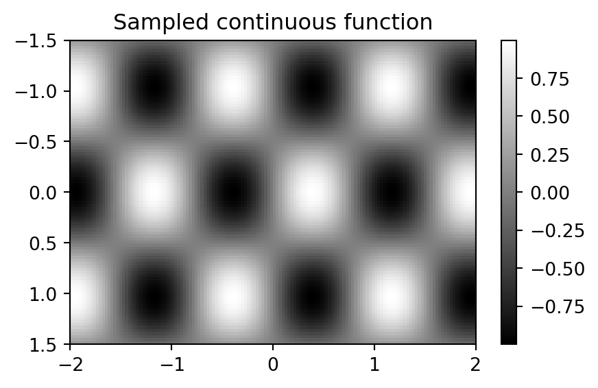
The extent argument tells Matplotlib which mathematical coordinates correspond to the image boundary.
7. Vectorization and Data Matrices
Many vision algorithms turn images into vectors.
vec = image.reshape(-1)
print(vec.shape)(9600,)A collection of images becomes a data matrix.
N = 20
images = []
for k in range(N):
    cx = rng.uniform(35, 85)
    cy = rng.uniform(25, 55)
    sigma = rng.uniform(10, 20)
    img = np.exp(-((X - cx)**2 + (Y - cy)**2) / (2 * sigma**2))
    images.append(img)

images = np.array(images)
X_data = images.reshape(N, -1)
print(images.shape)
print(X_data.shape)
(20, 100, 140)
(20, 14000)The data matrix convention used in many labs is:
\[ X \in \mathbb{R}^{N \times d}, \]
where \(N\) is the number of images or samples and \(d\) is the number of features.
8. Linear Algebra Tools
8.1 Norms, dot products, and distances
u = X_data[0]
v = X_data[1]

inner = np.dot(u, v)
norm_u = np.linalg.norm(u)
distance = np.linalg.norm(u - v)
cosine = inner / (np.linalg.norm(u) * np.linalg.norm(v))

print(inner, norm_u, distance, cosine)
535.5727980071915 30.83399953720921 27.777667277056917 0.5815727690245158Useful formulas:
\[ \|u\|_2 = \sqrt{\sum_i u_i^2}, \]
\[ \langle u,v \rangle = \sum_i u_i v_i, \]
\[ \cos(\theta) = \frac{\langle u,v \rangle}{\|u\|_2\|v\|_2}. \]
8.2 Least squares
Least squares solves
\[ \min_x \|Ax-b\|_2^2. \]
A = rng.normal(size=(30, 5))
x_true = rng.normal(size=5)
b = A @ x_true + 0.05 * rng.normal(size=30)

x_hat, residuals, rank, singular_values = np.linalg.lstsq(A, b, rcond=None)
print(x_hat)
print(np.linalg.norm(A @ x_hat - b))
[ 0.8028 0.9531 0.2636 0.3032 -0.214 ]
0.272959401177806048.3 SVD and PCA
X_centered = X_data - X_data.mean(axis=0, keepdims=True)
U, S, Vt = np.linalg.svd(X_centered, full_matrices=False)

print(U.shape, S.shape, Vt.shape)
(20, 20) (20,) (20, 14000)The rows of Vt are principal directions in feature space. The first few components often capture the main modes of variation in images.
9. Convolution and Filtering
9.1 Basic convolution filters
For small filters, scipy.ndimage.convolve is convenient.
mean_kernel = np.ones((5, 5)) / 25
smoothed = ndimage.convolve(image, mean_kernel, mode="reflect")
For derivative filters:
sobel_x = np.array([[-1, 0, 1],
                    [-2, 0, 2],
                    [-1, 0, 1]], dtype=float) / 8
sobel_y = sobel_x.T

Ix = ndimage.convolve(image, sobel_x, mode="reflect")
Iy = ndimage.convolve(image, sobel_y, mode="reflect")
grad_mag = np.sqrt(Ix**2 + Iy**2)
9.2 Gaussian smoothing
g = ndimage.gaussian_filter(image, sigma=2.0)The Gaussian is important because it reduces high-frequency noise before derivative estimation.
9.3 Boundary modes
Common boundary modes include:
reflect: mirror the image at the boundary.nearest: repeat the nearest boundary value.constant: pad with a constant value.wrap: use periodic boundary conditions.
Boundary handling can affect edges near the image border.
10. Fourier Analysis
10.1 Two-dimensional FFT
F = np.fft.fft2(image)
F_shift = np.fft.fftshift(F)
magnitude = np.log1p(np.abs(F_shift))

plt.figure(figsize=(5, 3))
plt.imshow(magnitude, cmap="gray")
plt.title("Log Fourier magnitude")
plt.axis("off")
plt.show()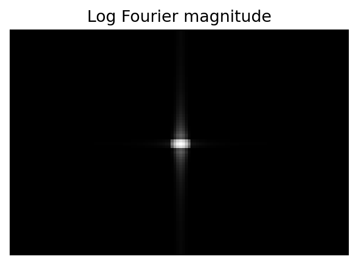
10.2 Low-pass filtering
H, W = image.shape
Y, X = np.mgrid[0:H, 0:W]
cy, cx = H // 2, W // 2
radius = 15
lowpass_mask = ((X - cx)**2 + (Y - cy)**2) <= radius**2

F_low = F_shift * lowpass_mask
image_low = np.real(np.fft.ifft2(np.fft.ifftshift(F_low)))
Fourier filtering is a numerical version of decomposing an image into frequencies.
11. Morphology and Connected Components
Binary morphology operates on masks.
mask = image > 0.35
opened = ndimage.binary_opening(mask, structure=np.ones((3, 3)))
closed = ndimage.binary_closing(opened, structure=np.ones((5, 5)))

labels, num_labels = ndimage.label(closed)
print(num_labels)1Connected components help separate individual objects in a binary segmentation mask.
sizes = ndimage.sum(closed, labels, index=np.arange(1, num_labels + 1))
print(sizes)[2145.]12. Geometry and Cameras
12.1 Homogeneous coordinates
A two-dimensional point \((x,y)\) becomes the homogeneous vector
\[ \tilde{x} = (x,y,1)^T. \]
points_2d = np.array([
    [10, 20],
    [50, 25],
    [80, 60]
], dtype=float)

points_h = np.c_[points_2d, np.ones(len(points_2d))]
print(points_h)
[[10. 20. 1.]
[50. 25. 1.]
[80. 60. 1.]]12.2 Projecting 3D points
A camera matrix maps homogeneous 3D points to homogeneous image points:
\[ \tilde{x} \sim P \tilde{X}. \]
def project_points(P, X3):
    Xh = np.c_[X3, np.ones(len(X3))]
    xh = (P @ Xh.T).T
    return xh[:, :2] / xh[:, 2:3]

K = np.array([[800, 0, 160],
              [0, 800, 120],
              [0, 0, 1]], dtype=float)
R = np.eye(3)
t = np.array([[0], [0], [0]], dtype=float)
P = K @ np.c_[R, t]

X3 = np.array([[0, 0, 4],
               [1, 0, 5],
               [0, 1, 6]], dtype=float)

x2 = project_points(P, X3)
print(x2)
[[160. 120. ]
[320. 120. ]
[160. 253.3333]]13. Optimization Tools
13.1 Scalar objective minimization
def objective(z):
    return (z[0] - 2)**2 + 0.5 * (z[1] + 1)**2

result = optimize.minimize(objective, x0=np.array([0.0, 0.0]))
print(result.x)
[ 2. -1.]13.2 Nonlinear least squares
Many geometry problems minimize reprojection residuals.
def residuals(theta):
    a, b = theta
    x = np.linspace(0, 1, 20)
    y_obs = 2.0 * x + 0.5 + 0.05 * rng.normal(size=x.shape)
    return a * x + b - y_obs

result = optimize.least_squares(residuals, x0=np.array([0.0, 0.0]))
print(result.x)
[-0. 0.]For bundle adjustment, calibration, and motion estimation, the residual vector usually contains many geometric errors.
14. Probability and Statistics
14.1 Random noise models
gaussian_noise = 0.1 * rng.normal(size=image.shape)
noisy_gaussian = image + gaussian_noise

poisson_counts = rng.poisson(20 * image)
noisy_poisson = poisson_counts / 20
Gaussian noise is common in continuous measurement models. Poisson noise appears in photon-counting models.
14.2 Histograms
plt.figure(figsize=(5, 3))
plt.hist(noisy_gaussian.ravel(), bins=40)
plt.title("Intensity histogram")
plt.xlabel("intensity")
plt.ylabel("count")
plt.show()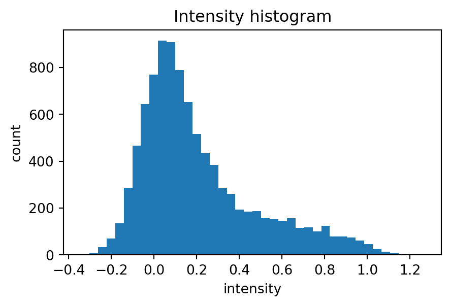
14.3 Classification metrics
y_true = np.array([0, 0, 1, 1, 1, 0])
y_pred = np.array([0, 1, 1, 1, 0, 0])

print(accuracy_score(y_true, y_pred))
print(confusion_matrix(y_true, y_pred))
0.6666666666666666
[[2 1]
[1 2]]In segmentation and detection labs, accuracy alone is often insufficient. IoU, Dice score, precision, recall, and average precision are more informative.
15. scikit-learn Patterns
15.1 Train/test split
X_small = rng.normal(size=(100, 8))
y_small = (X_small[:, 0] + 0.5 * X_small[:, 1] > 0).astype(int)

X_train, X_test, y_train, y_test = train_test_split(
    X_small, y_small, test_size=0.25, random_state=0, stratify=y_small
)

print(X_train.shape, X_test.shape)
(75, 8) (25, 8)15.2 PCA
from sklearn.decomposition import PCA

pca = PCA(n_components=2)
Z = pca.fit_transform(X_small)
print(Z.shape)
print(pca.explained_variance_ratio_)
(100, 2)
[0.1916 0.169 ]15.3 Logistic regression
from sklearn.linear_model import LogisticRegression

clf = LogisticRegression(max_iter=1000)
clf.fit(X_train, y_train)
y_hat = clf.predict(X_test)
print(accuracy_score(y_test, y_hat))1.016. TensorFlow Pattern for Optional Deep Learning Labs
Some later labs include optional TensorFlow sections for CNNs and modern vision models. A minimal pattern is:
try:
    import tensorflow as tf
    from tensorflow import keras
    print("TensorFlow version:", tf.__version__)
except Exception as e:
    print("TensorFlow is not available in this runtime.")
    print(e)
TensorFlow version: 2.15.0A small model may be created as follows.
try:
    import tensorflow as tf
    from tensorflow import keras

    model = keras.Sequential([
        keras.layers.Input(shape=(28, 28, 1)),
        keras.layers.Conv2D(8, 3, activation="relu"),
        keras.layers.MaxPooling2D(),
        keras.layers.Flatten(),
        keras.layers.Dense(10, activation="softmax")
    ])

    model.compile(
        optimizer="adam",
        loss="sparse_categorical_crossentropy",
        metrics=["accuracy"]
    )

    model.summary()
except Exception:
    pass
Model: "sequential"
_________________________________________________________________
Layer (type) Output Shape Param #
=================================================================
conv2d (Conv2D) (None, 26, 26, 8) 80
max_pooling2d (MaxPooling2 (None, 13, 13, 8) 0
D)
flatten (Flatten) (None, 1352) 0
dense (Dense) (None, 10) 13530
=================================================================
Total params: 13610 (53.16 KB)
Trainable params: 13610 (53.16 KB)
Non-trainable params: 0 (0.00 Byte)
_________________________________________________________________For independent study, students should understand the mathematical role of each layer before treating the model as a black box.
17. Useful Helper Functions
The following helper functions appear repeatedly in computer vision notebooks.
def show_image(img, title=None, cmap="gray", vmin=None, vmax=None, figsize=(5, 4)):
    plt.figure(figsize=figsize)
    if img.ndim == 2:
        plt.imshow(img, cmap=cmap, vmin=vmin, vmax=vmax)
    else:
        plt.imshow(np.clip(img, 0, 1))
    if title is not None:
        plt.title(title)
    plt.axis("off")
    plt.show()


def mse(a, b):
    a = np.asarray(a, dtype=float)
    b = np.asarray(b, dtype=float)
    return np.mean((a - b)**2)


def psnr(a, b, max_value=1.0, eps=1e-12):
    error = mse(a, b)
    return 10 * np.log10(max_value**2 / (error + eps))


def iou_score(mask_a, mask_b, eps=1e-12):
    mask_a = np.asarray(mask_a).astype(bool)
    mask_b = np.asarray(mask_b).astype(bool)
    intersection = np.logical_and(mask_a, mask_b).sum()
    union = np.logical_or(mask_a, mask_b).sum()
    return intersection / (union + eps)


def dice_score(mask_a, mask_b, eps=1e-12):
    mask_a = np.asarray(mask_a).astype(bool)
    mask_b = np.asarray(mask_b).astype(bool)
    intersection = np.logical_and(mask_a, mask_b).sum()
    return 2 * intersection / (mask_a.sum() + mask_b.sum() + eps)
18. Common Debugging Checklist
When a lab result looks wrong, check the following.
18.1 Shape errors
Print shapes early and often.
print("image shape:", image.shape)
print("data matrix shape:", X_data.shape)
image shape: (80, 120)
data matrix shape: (20, 14000)Typical mistakes:
- Confusing
(H, W)with(W, H). - Forgetting the channel dimension in RGB images.
- Flattening an image and then forgetting how to reshape it back.
- Mixing batches
(N, H, W, C)with single images(H, W, C).
18.2 Coordinate errors
Remember:
NumPy: image[row, column]
Math:  image[y, x]
In geometric vision, point coordinates are often stored as (x, y), but image arrays are indexed as [y, x].
18.3 Data type errors
Check whether the image is uint8 or float.
print(image_uint8.dtype)
print(image_float.dtype)
uint8
float64If an image has dtype uint8, arithmetic can behave unexpectedly. Convert to float before filtering, optimization, or learning.
18.4 Display errors
If an image looks blank, check the minimum and maximum.
print(image.min(), image.max())0.0003272810231830983 1.0Use normalization for visualization only when appropriate:
show_image(normalize01(image), title="Normalized for display")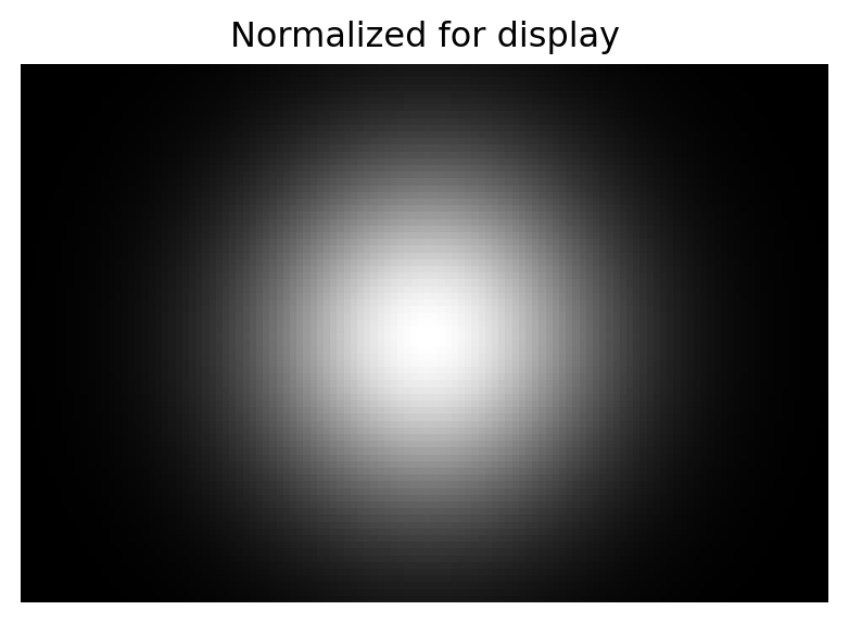
18.5 Randomness and reproducibility
Use a random generator:
rng = np.random.default_rng(2026)Avoid mixing too many random-number APIs in the same notebook.
19. Performance Tips for Colab
The labs are designed to run on standard Colab runtimes, but some experiments can become slow if array sizes are increased too much.
Useful habits:
- Start with small synthetic images such as
64 x 64or128 x 128. - Avoid Python loops over every pixel when vectorized NumPy or SciPy functions are available.
- Use
ndimageandsignalfor filtering instead of manually nested loops. - Use smaller training epochs when first checking a model.
- Save expensive model training for optional extensions or final projects.
- Restart the runtime if memory becomes unstable.
20. How to Study With This Reference
When working through a lab, use this page in three ways:
- Before coding: identify the array shapes and mathematical objects involved.
- While coding: compare your implementation with the short reference patterns.
- After coding: explain what each array represents mathematically.
The most important skill is not memorizing syntax. The most important skill is translating clearly between mathematics and computation:
\[ \text{mathematical model} \quad \longleftrightarrow \quad \text{array computation} \quad \longleftrightarrow \quad \text{visual result}. \]
That translation is the foundation of modern computer vision.