---
title: "Chapter 1. The First Language: Systems, Sets, and Structure"
subtitle: "From ordinary equations to the grammar of linear algebra"
format:
html:
toc: true
toc-depth: 3
number-sections: true
code-fold: show
code-tools: true
html-math-method: mathjax
pdf:
toc: true
number-sections: true
jupyter: python3
---
> **Guiding question.**
> How can many small equations become one geometric object, one computational problem, and one algebraic structure?
Linear algebra begins with a simple human problem: we know several pieces of information, and we want to find the unknowns.
At first this looks like algebra from high school:
$$
\begin{cases}
x+y=1,\\
x-y=3.
\end{cases}
$$
But in this book we will learn to see this system in several deeper ways.
It is a collection of equations.
It is an intersection of geometric objects.
It is a matrix equation.
It is a question about a function.
It is a problem over a field.
It is a computational task.
It is the first example of how linear algebra turns information into structure.
This chapter builds the language we need for the rest of the book. We begin with linear systems, then introduce sets, functions, algebraic objects, fields, and Gauss--Jordan elimination. These are not separate topics. They are the grammar of linear algebra.
::: {.callout-note title="How to read this chapter"}
This version keeps the story-driven style, but the definitions and theorems are written more precisely. The goal is to help you move between three levels:
1. intuition: what the idea means;
2. computation: how to calculate with it;
3. structure: why the theorem is true.
:::
::: {.callout-tip title="AI and coding companion"}
Students may use Python, MATLAB, or AI tools to check row reductions and explore examples. The purpose is not to replace mathematical thinking. The purpose is to ask precise questions, verify answers, find mistakes, and explain why a computation is correct.
:::
## 1.1 Linear systems as questions
We first fix a field $\mathbb F$. In this course the main examples are
$$
\mathbb R \quad \text{and} \quad \mathbb C.
$$
Most geometric examples in the beginning use $\mathbb R$, while later chapters on eigenvalues and Schur decomposition naturally use $\mathbb C$.
::: {.callout-note title="Definition 1.1: Linear equation"}
Let $\mathbb F$ be a field. A **linear equation** in the unknowns $x_1,x_2,\ldots,x_n$ over $\mathbb F$ is an equation of the form
$$
a_1x_1+a_2x_2+\cdots+a_nx_n=b,
$$
where $a_1,a_2,\ldots,a_n,b\in \mathbb F$ are fixed scalars and $x_1,x_2,\ldots,x_n$ are unknown scalars.
Equivalently, a linear equation is an equation in which each unknown appears only to the first power, and no products such as $x_ix_j$ occur.
:::
::: {.callout-note title="Definition 1.2: Linear system"}
A **linear system** of $m$ equations in $n$ unknowns over $\mathbb F$ is a collection of equations
$$
\begin{aligned}
a_{11}x_1+a_{12}x_2+\cdots+a_{1n}x_n &= b_1,\\
a_{21}x_1+a_{22}x_2+\cdots+a_{2n}x_n &= b_2,\\
&\vdots\\
a_{m1}x_1+a_{m2}x_2+\cdots+a_{mn}x_n &= b_m,
\end{aligned}
$$
where $a_{ij},b_i\in \mathbb F$.
A **solution** of the system is a vector
$$
\mathbf{x}=\begin{bmatrix}x_1\\x_2\\ \vdots\\x_n\end{bmatrix}\in \mathbb F^n
$$
such that all $m$ equations are satisfied.
The **solution set** is the subset of $\mathbb F^n$ consisting of all solutions.
:::
This system can be written as one matrix equation:
$$
A\mathbf{x}=\mathbf{b},
$$
where
$$
A=
\begin{bmatrix}
a_{11} & a_{12} & \cdots & a_{1n}\\
a_{21} & a_{22} & \cdots & a_{2n}\\
\vdots & \vdots & \ddots & \vdots\\
a_{m1} & a_{m2} & \cdots & a_{mn}
\end{bmatrix}\in \mathbb F^{m\times n},
\qquad
\mathbf{x}=
\begin{bmatrix}
x_1\\x_2\\ \vdots\\x_n
\end{bmatrix}\in \mathbb F^n,
\qquad
\mathbf{b}=
\begin{bmatrix}
b_1\\b_2\\ \vdots\\b_m
\end{bmatrix}\in \mathbb F^m.
$$
The matrix $A$ is called the **coefficient matrix**. The matrix
$$
[A\mid \mathbf b]
$$
is called the **augmented matrix**. It remembers both the coefficients and the target vector. It is the object we row-reduce.
::: {.callout-tip title="Story interpretation"}
Think of $A$ as a machine. The input is $\mathbf{x}$. The output is $A\mathbf{x}$. Solving $A\mathbf{x}=\mathbf b$ asks:
> Which inputs produce the desired output $\mathbf b$?
:::
## 1.2 The three possible endings
A linear system has only three possible types of solution sets:
1. no solution;
2. exactly one solution;
3. infinitely many solutions.
There is no fourth possibility.
::: {.callout-important title="Theorem 1.3: Trichotomy for linear systems"}
Let $A\in \mathbb F^{m\times n}$ and $\mathbf b\in \mathbb F^m$. The solution set of the linear system
$$
A\mathbf{x}=\mathbf b
$$
is exactly one of the following:
1. the empty set;
2. a set containing exactly one vector;
3. an infinite set.
More precisely, if the system is consistent and $\mathbf{x}_p$ is one particular solution, then the solution set is
$$
\mathbf{x}_p+\ker(A)=\{\mathbf{x}_p+\mathbf z: \mathbf z\in \ker(A)\}.
$$
Thus it has exactly one solution if $\ker(A)=\{\mathbf 0\}$ and infinitely many solutions if $\ker(A)\neq \{\mathbf 0\}$.
:::
::: {.callout-note title="Proof idea"}
If one solution $\mathbf{x}_p$ exists, then every other solution differs from $\mathbf{x}_p$ by a solution of the homogeneous system $A\mathbf z=\mathbf 0$. So the solution set is a translated copy of $\ker(A)$. A vector space is either the zero space or contains infinitely many vectors over $\mathbb R$ or $\mathbb C$.
:::
### Example: three systems in two unknowns
Consider the following systems over $\mathbb R$.
**No solution:**
$$
\begin{cases}
x+y=1,\\
x+y=2.
\end{cases}
$$
The two equations ask for the same left-hand side to equal two different numbers. Geometrically, these are two parallel lines.
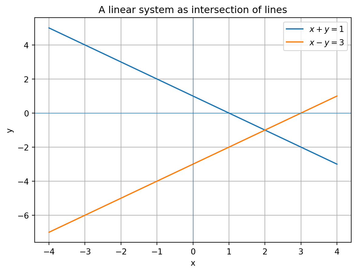
**One solution:**
$$
\begin{cases}
x+y=1,\\
x-y=3.
\end{cases}
$$
Adding the two equations gives $2x=4$, so $x=2$. Then $y=-1$. The solution is
$$
(x,y)=(2,-1).
$$
Geometrically, two nonparallel lines meet at one point.
**Infinitely many solutions:**
$$
\begin{cases}
x+y=1,\\
2x+2y=2.
\end{cases}
$$
The second equation is just twice the first. The solution set is the whole line
$$
(x,y)=(t,1-t),\qquad t\in\mathbb R.
$$
### Geometric view
In two variables, each nonzero linear equation is usually a line. In three variables, each nonzero linear equation is usually a plane. In higher dimensions, each nonzero linear equation defines a **hyperplane**.
Solving a linear system means finding an intersection.
That is the first geometric idea of linear algebra.
## 1.3 From equations to matrices
The system
$$
\begin{cases}
x+y=1,\\
x-y=3
\end{cases}
$$
can be written as
$$
\begin{bmatrix}
1 & 1\\
1 & -1
\end{bmatrix}
\begin{bmatrix}
x\\y
\end{bmatrix}
=
\begin{bmatrix}
1\\3
\end{bmatrix}.
$$
The augmented matrix is
$$
\left[
\begin{array}{cc|c}
1 & 1 & 1\\
1 & -1 & 3
\end{array}
\right].
$$
The matrix form is not just shorthand. It changes the problem. Once a system is written as a matrix equation, we can study it using row operations, functions, vector spaces, rank, geometry, numerical algorithms, and computation.
::: {.callout-note title="Definition 1.4: Matrix-vector product"}
Let $A=[a_{ij}]\in \mathbb F^{m\times n}$ and $\mathbf{x}=(x_1,\ldots,x_n)^T\in \mathbb F^n$. The product $A\mathbf{x}\in \mathbb F^m$ is defined by
$$
(A\mathbf{x})_i=\sum_{j=1}^n a_{ij}x_j,
\qquad i=1,\ldots,m.
$$
Equivalently, if $\mathbf a_1,\ldots,\mathbf a_n$ are the columns of $A$, then
$$
A\mathbf{x}=x_1\mathbf a_1+x_2\mathbf a_2+\cdots+x_n\mathbf a_n.
$$
:::
::: {.callout-important title="Column interpretation"}
The equation $A\mathbf{x}=\mathbf b$ asks whether $\mathbf b$ can be written as a linear combination of the columns of $A$.
:::
::: {.callout-note title="Why matrix notation matters"}
A matrix is not merely an array of numbers. It is a compressed description of a linear process.
:::
## 1.4 Sets: the language of collections
Before we go deeper, we need the language of sets.
::: {.callout-note title="Definition 1.5: Set"}
A **set** is a well-defined collection of distinct objects, called its **elements**.
If $x$ is an element of a set $S$, we write $x\in S$. If $x$ is not an element of $S$, we write $x\notin S$.
A set $A$ is a **subset** of a set $S$, written $A\subseteq S$, if every element of $A$ is also an element of $S$.
:::
Examples:
$$
\{1,2,3\},\qquad \mathbb R,\qquad \mathbb R^2,\qquad \{x\in\mathbb R:x^2<4\}.
$$
If $A$ and $B$ are subsets of a universe $S$, then:
$$
A\cup B=\{x\in S:x\in A\text{ or }x\in B\},
$$
$$
A\cap B=\{x\in S:x\in A\text{ and }x\in B\},
$$
$$
A^c=\{x\in S:x\notin A\}.
$$
::: {.callout-note title="Definition 1.6: Cartesian product"}
For sets $X$ and $Y$, the **Cartesian product** is
$$
X\times Y=\{(x,y):x\in X,\ y\in Y\}.
$$
For example, $\mathbb R\times\mathbb R=\mathbb R^2$.
:::
Later, vector spaces, matrix spaces, solution sets, subspaces, eigenspaces, function spaces, and Grassmannians will all be sets with additional structure.
## 1.5 Functions: the language of input and output
::: {.callout-note title="Definition 1.7: Function"}
Let $A$ and $B$ be sets. A **function** from $A$ to $B$ is a rule $f$ that assigns to each element $a\in A$ exactly one element $f(a)\in B$.
We write
$$
f:A\to B.
$$
The set $A$ is the **domain**. The set $B$ is the **codomain**. The **image** or **range** of $f$ is
$$
\operatorname{im}(f)=\{f(a):a\in A\}\subseteq B.
$$
:::
In linear algebra, the most important functions are linear maps:
$$
T:V\to W.
$$
A matrix is one way of representing a linear map.
### Injective, surjective, bijective
::: {.callout-note title="Definition 1.8: Injective, surjective, bijective"}
Let $f:A\to B$ be a function.
1. $f$ is **injective** or **one-to-one** if
$$
f(a_1)=f(a_2) \implies a_1=a_2
$$
for all $a_1,a_2\in A$.
2. $f$ is **surjective** or **onto** if
$$
\operatorname{im}(f)=B.
$$
Equivalently, for every $b\in B$, there exists $a\in A$ such that $f(a)=b$.
3. $f$ is **bijective** if it is both injective and surjective.
:::
For a linear map $T:V\to W$:
- injective means no information is lost;
- surjective means every target output can be reached;
- bijective means the process is perfectly reversible.
::: {.callout-tip title="Matrix translation"}
For a square matrix $A$, invertibility means the map $\mathbf{x}\mapsto A\mathbf{x}$ is bijective.
:::
## 1.6 Composition and inverse functions
::: {.callout-note title="Definition 1.9: Composition"}
Let
$$
f:A\to B,\qquad g:B\to C.
$$
The **composition** of $f$ followed by $g$ is the function
$$
g\circ f:A\to C
$$
defined by
$$
(g\circ f)(a)=g(f(a)).
$$
:::
In matrix language, composition of linear maps becomes matrix multiplication.
If $T(\mathbf{x})=A\mathbf{x}$ and $S(\mathbf{y})=B\mathbf{y}$, then
$$
(S\circ T)(\mathbf{x})=B(A\mathbf{x})=(BA)\mathbf{x}.
$$
This is why matrix multiplication appears in the order $BA$: first apply $A$, then apply $B$.
::: {.callout-note title="Definition 1.10: Inverse function"}
A function $f:A\to B$ is **invertible** if there exists a function $f^{-1}:B\to A$ such that
$$
f^{-1}(f(a))=a \quad \text{for all } a\in A,
$$
and
$$
f(f^{-1}(b))=b \quad \text{for all } b\in B.
$$
A function is invertible if and only if it is bijective.
:::
For matrices, this becomes
$$
A^{-1}A=I,
\qquad
AA^{-1}=I.
$$
## 1.7 Algebraic objects: operations with rules
Linear algebra is not only about numbers. It is about operations that obey rules.
::: {.callout-note title="Definition 1.11: Binary operation"}
A **binary operation** on a set $S$ is a function
$$
*:S\times S\to S.
$$
For $a,b\in S$, the output is usually written $a*b$.
:::
Examples:
- addition on $\mathbb R$;
- multiplication on $\mathbb R$;
- matrix addition on $\mathbb R^{m\times n}$;
- matrix multiplication on $\mathbb R^{n\times n}$.
A set with an operation may have algebraic structure.
### Monoids
::: {.callout-note title="Definition 1.12: Monoid"}
A **monoid** is a set $M$ together with a binary operation $*$ such that:
1. **associativity:** $(a*b)*c=a*(b*c)$ for all $a,b,c\in M$;
2. **identity:** there exists an element $e\in M$ such that $e*a=a*e=a$ for all $a\in M$.
:::
Square matrices under multiplication form a monoid:
$$
A(BC)=(AB)C,
\qquad
AI=IA=A.
$$
Not every matrix has a multiplicative inverse, so this is not a group.
### Groups
::: {.callout-note title="Definition 1.13: Group"}
A **group** is a set $G$ together with a binary operation $*$ such that:
1. **closure:** $a*b\in G$ for all $a,b\in G$;
2. **associativity:** $(a*b)*c=a*(b*c)$ for all $a,b,c\in G$;
3. **identity:** there exists $e\in G$ such that $e*a=a*e=a$ for all $a\in G$;
4. **inverse:** for every $a\in G$, there exists $a^{-1}\in G$ such that $a*a^{-1}=a^{-1}*a=e$.
If also $a*b=b*a$ for all $a,b\in G$, then $G$ is an **abelian group**.
:::
The set of all invertible $n\times n$ matrices over a field $\mathbb F$ is called the **general linear group**:
$$
GL(n,\mathbb F)=\{A\in \mathbb F^{n\times n}:A\text{ is invertible}\}.
$$
This group will appear naturally whenever we study change of basis.
### Rings and fields
::: {.callout-note title="Definition 1.14: Ring"}
A **ring** is a set $R$ with two operations, addition and multiplication, such that:
1. $(R,+)$ is an abelian group;
2. multiplication is associative;
3. multiplication distributes over addition:
$$
a(b+c)=ab+ac, \qquad (a+b)c=ac+bc.
$$
Some authors require a multiplicative identity in the definition of a ring. In this book, when a multiplicative identity is needed, we will say so explicitly.
:::
::: {.callout-note title="Definition 1.15: Field"}
A **field** is a set $\mathbb F$ with two operations, addition and multiplication, such that:
1. $(\mathbb F,+)$ is an abelian group with additive identity $0$;
2. $\mathbb F\setminus\{0\}$ is an abelian group under multiplication with multiplicative identity $1$;
3. multiplication distributes over addition.
In a field, addition, subtraction, multiplication, and division by nonzero elements are all possible.
:::
Important examples:
$$
\mathbb Q,
\qquad
\mathbb R,
\qquad
\mathbb C.
$$
The rational numbers, real numbers, and complex numbers are fields.
The integers $\mathbb Z$ are not a field because, for example, $2$ has no multiplicative inverse inside $\mathbb Z$.
::: {.callout-warning title="Fields matter"}
Many theorems in linear algebra depend on the field. A matrix may have real eigenvalues over $\mathbb R$, or only complex eigenvalues over $\mathbb C$. Later, this difference becomes important in spectral theory and Schur decomposition.
:::
## 1.8 Gauss--Jordan elimination
The main computational method for solving linear systems is row reduction.
::: {.callout-note title="Definition 1.16: Elementary row operations"}
The three **elementary row operations** on a matrix are:
1. interchange two rows;
2. multiply one row by a nonzero scalar;
3. replace one row by itself plus a scalar multiple of another row.
These operations are performed on the augmented matrix of a linear system.
:::
::: {.callout-important title="Theorem 1.17: Row operations preserve solution sets"}
Elementary row operations on the augmented matrix of a linear system do not change the solution set of the system.
:::
::: {.callout-note title="Proof idea"}
Each row represents one equation. Swapping equations does not change the set of common solutions. Multiplying an equation by a nonzero scalar gives an equivalent equation. Replacing one equation by itself plus a multiple of another equation also gives an equivalent system because the operation can be reversed.
:::
The goal is to transform the augmented matrix into a simpler matrix.
### Row-echelon and reduced row-echelon form
::: {.callout-note title="Definition 1.18: Pivot and row-echelon form"}
Let $M$ be a matrix. The **leading entry** of a nonzero row is the first nonzero entry in that row, reading from left to right. A **pivot position** is the position of a leading entry in a row-echelon form of $M$.
A matrix is in **row-echelon form** if:
1. all zero rows, if any, are below all nonzero rows;
2. the leading entry of each nonzero row is strictly to the right of the leading entry of the row above it;
3. all entries below each leading entry are zero.
:::
::: {.callout-note title="Definition 1.19: Reduced row-echelon form"}
A matrix is in **reduced row-echelon form** if it is in row-echelon form and, in addition:
1. each leading entry is equal to $1$;
2. each leading $1$ is the only nonzero entry in its column.
The reduced row-echelon form of a matrix $M$ is denoted by $\operatorname{rref}(M)$.
:::
::: {.callout-important title="Theorem 1.20: Uniqueness of reduced row-echelon form"}
Every matrix over a field is row equivalent to exactly one reduced row-echelon matrix.
:::
The leading variables are called **pivot variables**. The remaining variables are **free variables**.
## 1.9 A worked example
Solve
$$
\begin{cases}
x+y+z=2,\\
2x+3y+z=5,\\
x+2y+3z=6.
\end{cases}
$$
The augmented matrix is
$$
\left[
\begin{array}{ccc|c}
1&1&1&2\\
2&3&1&5\\
1&2&3&6
\end{array}
\right].
$$
Perform row operations:
$$
\left[
\begin{array}{ccc|c}
1&1&1&2\\
2&3&1&5\\
1&2&3&6
\end{array}
\right]
\xrightarrow{R_2\leftarrow R_2-2R_1,\ R_3\leftarrow R_3-R_1}
\left[
\begin{array}{ccc|c}
1&1&1&2\\
0&1&-1&1\\
0&1&2&4
\end{array}
\right].
$$
Then
$$
\left[
\begin{array}{ccc|c}
1&1&1&2\\
0&1&-1&1\\
0&1&2&4
\end{array}
\right]
\xrightarrow{R_3\leftarrow R_3-R_2}
\left[
\begin{array}{ccc|c}
1&1&1&2\\
0&1&-1&1\\
0&0&3&3
\end{array}
\right]
\xrightarrow{R_3\leftarrow \frac13R_3}
\left[
\begin{array}{ccc|c}
1&1&1&2\\
0&1&-1&1\\
0&0&1&1
\end{array}
\right].
$$
Back substitution gives
$$
z=1,
\qquad
y-z=1,
\qquad
x+y+z=2.
$$
Thus
$$
z=1,
\qquad
y=2,
\qquad
x=-1.
$$
So the solution is
$$
\mathbf{x}=
\begin{bmatrix}
-1\\2\\1
\end{bmatrix}.
$$
## 1.10 Rank, consistency, and free variables
::: {.callout-note title="Definition 1.21: Rank"}
The **rank** of a matrix $A$, denoted $\operatorname{rank}(A)$, is the number of pivot columns in a row-echelon form of $A$.
Equivalently, $\operatorname{rank}(A)$ is the dimension of the column space of $A$.
:::
For a system
$$
A\mathbf{x}=\mathbf b,
$$
we compare the rank of $A$ and the rank of the augmented matrix $[A\mid \mathbf b]$.
::: {.callout-important title="Theorem 1.22: Rank criterion for consistency"}
Let $A\in \mathbb F^{m\times n}$ and $\mathbf b\in \mathbb F^m$. The system
$$
A\mathbf{x}=\mathbf b
$$
is consistent if and only if
$$
\operatorname{rank}(A)=\operatorname{rank}([A\mid \mathbf b]).
$$
:::
::: {.callout-note title="Proof idea"}
The augmented matrix has one additional column, the vector $\mathbf b$. If adding this column creates a new pivot, then $\mathbf b$ is not generated by the columns of $A$, and the system is inconsistent. If it does not create a new pivot, then $\mathbf b$ lies in the column space of $A$, and the system is consistent.
:::
::: {.callout-important title="Theorem 1.23: Counting free variables"}
Assume $A\mathbf{x}=\mathbf b$ is consistent, where $A\in \mathbb F^{m\times n}$. Then
$$
\text{number of free variables}=n-\operatorname{rank}(A).
$$
Therefore:
1. if $\operatorname{rank}(A)=\operatorname{rank}([A\mid \mathbf b])=n$, there is a unique solution;
2. if $\operatorname{rank}(A)=\operatorname{rank}([A\mid \mathbf b])<n$, there are infinitely many solutions over $\mathbb R$ or $\mathbb C$;
3. if $\operatorname{rank}(A)<\operatorname{rank}([A\mid \mathbf b])$, there is no solution.
:::
## 1.11 The deeper view: matrix equations as linear maps
::: {.callout-note title="Definition 1.24: Linear map"}
Let $V$ and $W$ be vector spaces over the same field $\mathbb F$. A function $T:V\to W$ is called **linear** if, for all $\mathbf u,\mathbf v\in V$ and all scalars $c\in \mathbb F$,
$$
T(\mathbf u+\mathbf v)=T(\mathbf u)+T(\mathbf v),
$$
and
$$
T(c\mathbf u)=cT(\mathbf u).
$$
Equivalently,
$$
T(c_1\mathbf v_1+c_2\mathbf v_2)=c_1T(\mathbf v_1)+c_2T(\mathbf v_2)
$$
for all $\mathbf v_1,\mathbf v_2\in V$ and $c_1,c_2\in\mathbb F$.
:::
Every matrix $A\in\mathbb F^{m\times n}$ defines a linear map
$$
T_A:\mathbb F^n\to\mathbb F^m,
\qquad
T_A(\mathbf{x})=A\mathbf{x}.
$$
::: {.callout-note title="Definition 1.25: Image, column space, and kernel"}
For $A\in \mathbb F^{m\times n}$, define
$$
\operatorname{Col}(A)=\operatorname{im}(T_A)=\{A\mathbf{x}:\mathbf{x}\in\mathbb F^n\}\subseteq \mathbb F^m,
$$
and
$$
\ker(A)=\{\mathbf{x}\in\mathbb F^n:A\mathbf{x}=\mathbf 0\}\subseteq \mathbb F^n.
$$
The space $\operatorname{Col}(A)$ is called the **column space** of $A$. The space $\ker(A)$ is called the **kernel** or **null space** of $A$.
:::
Therefore
$$
A\mathbf{x}=\mathbf b
$$
has a solution if and only if
$$
\mathbf b\in \operatorname{Col}(A).
$$
This is one of the most important conceptual shifts in linear algebra.
We stop asking only:
> Can I solve the equations?
We start asking:
> Is the target vector inside the space generated by the columns?
## 1.12 Affine structure of solution sets
::: {.callout-important title="Theorem 1.26: Structure of the solution set"}
Let $A\in\mathbb F^{m\times n}$ and $\mathbf b\in\mathbb F^m$. Suppose $\mathbf{x}_p$ is one solution of
$$
A\mathbf{x}=\mathbf b.
$$
Then the full solution set is
$$
\mathbf{x}_p+\ker(A)=\{\mathbf{x}_p+\mathbf z:\mathbf z\in\ker(A)\}.
$$
In words, every solution is one particular solution plus a solution of the homogeneous system $A\mathbf z=\mathbf 0$.
:::
::: {.callout-note title="Proof"}
Let $\mathbf{x}$ be any solution. Then
$$
A\mathbf{x}=\mathbf b,
\qquad
A\mathbf{x}_p=\mathbf b.
$$
Subtracting gives
$$
A(\mathbf{x}-\mathbf{x}_p)=\mathbf 0.
$$
Thus $\mathbf{x}-\mathbf{x}_p\in\ker(A)$, so $\mathbf{x}=\mathbf{x}_p+\mathbf z$ for some $\mathbf z\in\ker(A)$.
Conversely, if $\mathbf z\in\ker(A)$, then
$$
A(\mathbf{x}_p+\mathbf z)=A\mathbf{x}_p+A\mathbf z=\mathbf b+\mathbf 0=\mathbf b.
$$
So every vector of the form $\mathbf{x}_p+\mathbf z$ is a solution.
:::
This is an **affine subspace**: a translated version of the null space.
::: {.callout-note title="Key idea"}
Solving a nonhomogeneous system means finding one particular solution and then adding all solutions of the homogeneous system.
:::
## 1.13 Computation lab: row reduction in Python
We now use Python to solve the worked example.
```{python}
import sympy as sp

A = sp.Matrix([
    [1, 1, 1],
    [2, 3, 1],
    [1, 2, 3]
])

b = sp.Matrix([2, 5, 6])

Aug = A.row_join(b)
Aug_rref, pivots = Aug.rref()

Aug_rref, pivots
```
The reduced row-echelon form tells us the solution directly.
```{python}
solution = A.LUsolve(b)
solution
```
We can also check the answer.
```{python}
A * solution
```
### Numerical version with NumPy
```{python}
import numpy as np

A_np = np.array([
    [1, 1, 1],
    [2, 3, 1],
    [1, 2, 3]
], dtype=float)

b_np = np.array([2, 5, 6], dtype=float)

x_np = np.linalg.solve(A_np, b_np)
x_np
```
::: {.callout-warning title="Symbolic vs numerical computation"}
`sympy` performs exact symbolic computation when possible. `numpy` performs numerical computation using floating-point arithmetic. In small examples they often agree, but for large or ill-conditioned systems, numerical issues become important.
:::
### A quick rank test in Python
```{python}
A = sp.Matrix([
    [1, 2, 1],
    [2, 4, 2],
    [1, 1, 0]
])

b = sp.Matrix([3, 6, 1])
Aug = A.row_join(b)

A.rank(), Aug.rank(), Aug.rref()
```
The pair
$$
\bigl(\operatorname{rank}(A),\operatorname{rank}([A\mid \mathbf b])\bigr)
$$
tells us whether the system is consistent.
## 1.14 AI companion: use AI, but verify
Students now have access to AI tools. This changes how we study linear algebra.
AI can help generate examples, explain steps, and write code. But AI can also make mistakes, skip assumptions, or confuse similar concepts.
Here is a useful prompt:
> Explain why elementary row operations do not change the solution set of a linear system. Give a numerical example and a geometric interpretation.
After reading the answer, check:
1. Did it explain all three row operations?
2. Did it distinguish changing equations from changing solutions?
3. Did it use a correct example?
4. Did it mention that multiplying a row by zero is not allowed?
5. Can you rewrite the explanation in your own words?
::: {.callout-tip title="Responsible AI habit"}
Do not ask AI only for the answer. Ask it for examples, counterexamples, visualizations, and alternative explanations. Then verify the mathematics yourself.
:::
## 1.15 Mini-project: systems as intersections
Choose one of the following systems:
$$
\begin{cases}
x+y=1,\\
x-y=3,
\end{cases}
\qquad
\begin{cases}
x+y=1,\\
2x+2y=2,
\end{cases}
\qquad
\begin{cases}
x+y=1,\\
x+y=2.
\end{cases}
$$
For your chosen system:
1. Write the augmented matrix.
2. Row-reduce it.
3. Describe the solution set algebraically.
4. Describe the solution set geometrically.
5. Use Python to plot the two lines.
6. Ask AI to explain the result, then critique its explanation.
Here is starter code.
```{python}
import numpy as np
import matplotlib.pyplot as plt

x = np.linspace(-4, 4, 400)

# Example: x + y = 1 and x - y = 3
y1 = 1 - x
y2 = x - 3

plt.figure()
plt.plot(x, y1, label=r"$x+y=1$")
plt.plot(x, y2, label=r"$x-y=3$")
plt.axhline(0, linewidth=0.5)
plt.axvline(0, linewidth=0.5)
plt.xlabel("x")
plt.ylabel("y")
plt.legend()
plt.title("A linear system as intersection of lines")
plt.grid(True)
plt.show()
```
## 1.16 Chapter summary
This chapter introduced the first language of linear algebra.
We learned that:
- a linear system can be written as $A\mathbf{x}=\mathbf b$;
- the augmented matrix $[A\mid \mathbf b]$ contains the data of the system;
- a linear system has no solution, one solution, or infinitely many solutions;
- sets and functions provide the language for later mathematical structures;
- algebraic objects such as groups, rings, and fields explain the rules of computation;
- Gauss--Jordan elimination solves systems by elementary row operations;
- rank detects consistency and free variables;
- the equation $A\mathbf{x}=\mathbf b$ asks whether $\mathbf b$ lies in the column space of $A$;
- if one solution exists, all solutions form $\mathbf{x}_p+\ker(A)$;
- AI and coding are useful companions, but mathematical verification is essential.
The next chapter begins the study of vectors and vector spaces. We will move from systems of equations to the spaces of all possible solutions.
## Exercises
### Conceptual exercises
1. Explain why a system of two linear equations in two variables cannot have exactly two solutions.
2. Give an example of a system with infinitely many solutions. Explain both algebraically and geometrically.
3. What is the difference between the coefficient matrix and the augmented matrix?
4. Explain why the equation $A\mathbf{x}=\mathbf b$ has a solution if and only if $\mathbf b$ is in the column space of $A$.
5. Why is multiplying a row by zero not an elementary row operation?
### Computational exercises
6. Solve the system
$$
\begin{cases}
2x+3y=4,\\
x-y=1.
\end{cases}
$$
7. Decide whether the following system is consistent:
$$
\begin{cases}
x+2y+z=1,\\
2x+4y+2z=3.
\end{cases}
$$
8. Row-reduce the augmented matrix
$$
\left[
\begin{array}{ccc|c}
1&2&1&3\\
2&4&2&6\\
1&1&0&1
\end{array}
\right].
$$
Determine the solution set.
9. Find the rank of
$$
A=
\begin{bmatrix}
1&2&3\\
2&4&6\\
1&1&1
\end{bmatrix}.
$$
10. For the matrix in Exercise 9, determine whether the columns are linearly independent.
### Proof exercises
11. Prove that swapping two equations in a linear system does not change the solution set.
12. Prove that if $\mathbf{x}_p$ is one solution of $A\mathbf{x}=\mathbf b$, then every solution has the form
$$
\mathbf{x}_p+\mathbf{x}_h,
$$
where $A\mathbf{x}_h=\mathbf 0$.
13. Prove that if $A$ is an invertible square matrix, then $A\mathbf{x}=\mathbf b$ has a unique solution for every $\mathbf b$.
### Coding exercises
14. Write a Python function that takes an augmented matrix and returns its reduced row-echelon form using `sympy`.
15. Generate three random $3\times 3$ matrices. For each matrix, compute its rank and determinant. What do you observe when the determinant is zero?
16. Use Python to create a system with infinitely many solutions. Row-reduce the augmented matrix and identify the free variables.
### AI companion exercises
17. Ask an AI tool:
“What is the relationship between rank and the number of solutions of a linear system?”
Then critique the answer. Did it mention the augmented matrix?
18. Ask an AI tool to produce a system with no solution, one solution, and infinitely many solutions. Verify each example by row reduction.
19. Ask an AI tool to explain the difference between symbolic and numerical computation. Then test its explanation by solving a system using both `sympy` and `numpy`.
## Selected solutions
### Solution to Exercise 1
Two distinct lines in the plane either do not meet, meet once, or are the same line. If they are the same line, they share infinitely many points. Therefore two linear equations in two variables cannot have exactly two solutions.
### Solution to Exercise 6
From
$$
\begin{cases}
2x+3y=4,\\
x-y=1,
\end{cases}
$$
the second equation gives $x=y+1$. Substitute into the first:
$$
2(y+1)+3y=4.
$$
So
$$
5y+2=4,
\qquad
5y=2,
\qquad
y=\frac25.
$$
Then
$$
x=1+\frac25=\frac75.
$$
Thus
$$
(x,y)=\left(\frac75,\frac25\right).
$$
### Solution to Exercise 12
Suppose $\mathbf{x}$ is any solution of $A\mathbf{x}=\mathbf b$ and $\mathbf{x}_p$ is one particular solution. Then
$$
A\mathbf{x}=\mathbf b,
\qquad
A\mathbf{x}_p=\mathbf b.
$$
Subtracting gives
$$
A(\mathbf{x}-\mathbf{x}_p)=\mathbf 0.
$$
Thus $\mathbf{x}-\mathbf{x}_p\in\ker(A)$, so
$$
\mathbf{x}=\mathbf{x}_p+\mathbf{x}_h
$$
for some $\mathbf{x}_h\in\ker(A)$.
Conversely, if $\mathbf{x}_h\in\ker(A)$, then
$$
A(\mathbf{x}_p+\mathbf{x}_h)=A\mathbf{x}_p+A\mathbf{x}_h=\mathbf b+\mathbf 0=\mathbf b.
$$
Therefore every vector of the form $\mathbf{x}_p+\mathbf{x}_h$ is a solution.