---
title: "Chapter 14: Singular Value Decomposition"
subtitle: "Every Matrix Has a Geometry"
author: "He Wang"
format:
html:
toc: true
number-sections: true
code-fold: true
code-tools: true
theme: cosmo
execute:
echo: true
warning: false
message: false
jupyter: python3
---
## The story: the spectral theorem grows up
In Chapter 13, symmetric and Hermitian matrices gave us a beautiful story:
$$
A = QDQ^T
\qquad \text{or} \qquad
A = UDU^*.
$$
A symmetric matrix acts by choosing orthogonal directions, stretching each direction by an eigenvalue, and then recombining the result. This is one of the cleanest geometric pictures in linear algebra.
But most matrices in applications are not symmetric. Many are not even square. A data matrix may have rows representing people and columns representing features. An image is a rectangular grid of pixel intensities. A machine-learning design matrix may have thousands of observations and hundreds of variables.
The **singular value decomposition**, or **SVD**, says that every matrix still has a spectral-type geometry. The matrix may not have enough eigenvectors, but it always has singular vectors.
The central idea is simple:
> To understand a general matrix $X$, study the symmetric positive semidefinite matrix $X^T X$.
This chapter develops SVD from this idea and then connects it to geometry, matrix norms, pseudoinverses, least squares, image compression, and principal component analysis.
## Learning goals
After this chapter, you should be able to:
1. define singular values and singular vectors;
2. derive the singular value decomposition from the spectral theorem for $X^T X$;
3. compute SVD numerically in Python;
4. interpret SVD geometrically as rotation/reflection, scaling, and rotation/reflection;
5. use singular values to compute rank and the spectral norm;
6. use SVD to form low-rank approximations and pseudoinverses;
7. explain why SVD is important in least squares, image compression, and PCA.
## 14.1 The Gram matrix $X^T X$
Let $X\in \mathbb R^{N\times d}$. The columns of $X$ are vectors in $\mathbb R^N$. The matrix $X^T X$ records all dot products among these columns.
::: {.callout-note}
## Definition 14.1: Gram matrix
Let $X\in \mathbb R^{N\times d}$. The matrix
$$
G=X^T X\in \mathbb R^{d\times d}
$$
is called the **Gram matrix** of $X$.
:::
The Gram matrix is always symmetric:
$$
(X^T X)^T = X^T X.
$$
It is also positive semidefinite, because for every vector $v\in \mathbb R^d$,
$$
v^T X^T X v = (Xv)^T(Xv)=\|Xv\|_2^2\ge 0.
$$
::: {.callout-important}
## Proposition 14.2: Basic properties of $X^T X$
Let $X\in\mathbb R^{N\times d}$. Then:
1. $X^T X$ is symmetric.
2. $X^T X$ is positive semidefinite.
3. $\ker(X^T X)=\ker(X)$.
4. $\operatorname{rank}(X^T X)=\operatorname{rank}(X)$.
:::
<details>
<summary>Proof</summary>
Symmetry follows from
$$
(X^T X)^T=X^T(X^T)^T=X^T X.
$$
For positive semidefiniteness, compute
$$
v^T X^T Xv=\|Xv\|_2^2\ge 0.
$$
If $Xv=0$, then clearly $X^T Xv=0$. Conversely, if $X^T Xv=0$, then
$$
0=v^T X^T Xv=\|Xv\|_2^2,
$$
so $Xv=0$. Thus the kernels are equal. Rank-nullity gives
$$
\operatorname{rank}(X^T X)
=d-\dim\ker(X^T X)
=d-\dim\ker(X)
=\operatorname{rank}(X).
$$
</details>
## 14.2 Singular values
Since $X^T X$ is symmetric positive semidefinite, the spectral theorem applies. Therefore $X^T X$ has an orthonormal eigenbasis and nonnegative eigenvalues.
Suppose
$$
X^T X v_i=\lambda_i v_i,
$$
where
$$
\lambda_1\ge \lambda_2\ge\cdots\ge \lambda_p>0=\lambda_{p+1}=\cdots=\lambda_d.
$$
The **singular values** of $X$ are the square roots of the eigenvalues of $X^T X$:
$$
\sigma_i=\sqrt{\lambda_i}.
$$
::: {.callout-note}
## Definition 14.3: Singular values
Let $X\in\mathbb R^{N\times d}$. The singular values of $X$ are
$$
\sigma_i=\sqrt{\lambda_i},
$$
where $\lambda_i$ are the eigenvalues of $X^T X$, listed in nonincreasing order. Thus
$$
\sigma_1\ge\sigma_2\ge\cdots\ge\sigma_p>0.
$$
The rank of $X$ is the number of nonzero singular values.
:::
The eigenvectors $v_i$ of $X^T X$ are called **right singular vectors**. For each positive singular value, define
$$
u_i=\frac{Xv_i}{\|Xv_i\|_2}=\frac{Xv_i}{\sigma_i}.
$$
These vectors are called **left singular vectors**.
::: {.callout-important}
## Lemma 14.4: Orthogonality of left singular vectors
For $i,j\in\{1,\ldots,p\}$,
$$
\langle u_i,u_j\rangle=\delta_{ij}.
$$
:::
<details>
<summary>Proof</summary>
Using $u_i=Xv_i/\sigma_i$, we compute
$$
\langle u_i,u_j\rangle
=\frac{1}{\sigma_i\sigma_j}(Xv_i)^T(Xv_j)
=\frac{1}{\sigma_i\sigma_j}v_i^T X^T X v_j.
$$
Since $X^T Xv_j=\sigma_j^2v_j$,
$$
\langle u_i,u_j\rangle
=\frac{\sigma_j^2}{\sigma_i\sigma_j}v_i^T v_j
=\frac{\sigma_j}{\sigma_i}\delta_{ij}.
$$
If $i=j$, this equals $1$. If $i\ne j$, this equals $0$.
</details>
## 14.3 The singular value decomposition
Let
$$
U=[u_1\ \cdots\ u_N],
\qquad
V=[v_1\ \cdots\ v_d]
$$
be orthogonal matrices obtained by completing the left and right singular vectors to orthonormal bases. Let $\Sigma$ be the rectangular diagonal matrix whose diagonal entries are the singular values.
::: {.callout-important}
## Theorem 14.5: Singular value decomposition
For every matrix $X\in\mathbb R^{N\times d}$ of rank $p$, there exist orthogonal matrices
$$
U\in\mathbb R^{N\times N},
\qquad
V\in\mathbb R^{d\times d},
$$
and a rectangular diagonal matrix $\Sigma\in\mathbb R^{N\times d}$ such that
$$
X=U\Sigma V^T.
$$
Equivalently,
$$
X=\sigma_1u_1v_1^T+\sigma_2u_2v_2^T+\cdots+\sigma_pu_pv_p^T.
$$
:::
<details>
<summary>Proof</summary>
For $i=1,\ldots,p$, the definition of $u_i$ gives
$$
Xv_i=\sigma_i u_i.
$$
For $i=p+1,\ldots,d$, the eigenvalue of $X^T X$ is $0$, so
$$
0=v_i^T X^T Xv_i=\|Xv_i\|_2^2.
$$
Therefore $Xv_i=0$. Hence
$$
XV=[Xv_1\ \cdots\ Xv_d]
=[\sigma_1u_1\ \cdots\ \sigma_pu_p\ 0\ \cdots\ 0]
=U\Sigma.
$$
Multiplying by $V^T$ on the right gives
$$
X=U\Sigma V^T.
$$
The rank-one expansion follows by multiplying out $U\Sigma V^T$.
</details>
::: {.callout-tip}
## Interpretation
The SVD says that every linear transformation can be decomposed as
$$
X=U\Sigma V^T.
$$
Read this from right to left:
1. $V^T$ rotates or reflects the input space.
2. $\Sigma$ scales along coordinate directions.
3. $U$ rotates or reflects the output space.
:::
## 14.4 Compact and truncated SVD
The full SVD may contain many zero singular values. In computation, we often keep only the nonzero part.
::: {.callout-note}
## Definition 14.6: Compact SVD
Let $X\in\mathbb R^{N\times d}$ have rank $p$. The compact SVD is
$$
X=U_p\Sigma_pV_p^T,
$$
where
$$
U_p=[u_1\ \cdots\ u_p],
\qquad
V_p=[v_1\ \cdots\ v_p],
\qquad
\Sigma_p=\operatorname{diag}(\sigma_1,\ldots,\sigma_p).
$$
:::
::: {.callout-note}
## Definition 14.7: Rank-$k$ truncation
For $1\le k\le p$, the rank-$k$ truncation of $X$ is
$$
X_k=\sigma_1u_1v_1^T+\cdots+\sigma_ku_kv_k^T.
$$
This keeps the first $k$ singular directions and discards the remaining ones.
:::
## 14.5 Example: computing an SVD by hand
Consider
$$
M=\begin{bmatrix}
0&1&1\\
1&1&0
\end{bmatrix}.
$$
Then
$$
M^TM=
\begin{bmatrix}
1&1&0\\
1&2&1\\
0&1&1
\end{bmatrix}.
$$
The eigenvalues of $M^TM$ are $3,1,0$. Therefore the singular values are
$$
\sigma_1=\sqrt3,
\qquad
\sigma_2=1.
$$
One possible orthonormal eigenbasis is
$$
v_1=\frac{1}{\sqrt6}\begin{bmatrix}1\\2\\1\end{bmatrix},
\qquad
v_2=\frac{1}{\sqrt2}\begin{bmatrix}1\\0\\-1\end{bmatrix},
\qquad
v_3=\frac{1}{\sqrt3}\begin{bmatrix}1\\-1\\1\end{bmatrix}.
$$
Then
$$
u_1=\frac{Mv_1}{\sqrt3}=\frac{1}{\sqrt2}\begin{bmatrix}1\\1\end{bmatrix},
\qquad
u_2=Mv_2=\frac{1}{\sqrt2}\begin{bmatrix}-1\\1\end{bmatrix}.
$$
Thus one SVD is
$$
M=U\Sigma V^T,
$$
where
$$
U=\frac{1}{\sqrt2}
\begin{bmatrix}
1&-1\\
1&1
\end{bmatrix},
\qquad
\Sigma=
\begin{bmatrix}
\sqrt3&0&0\\
0&1&0
\end{bmatrix},
$$
and
$$
V=
\begin{bmatrix}
1/\sqrt6&1/\sqrt2&1/\sqrt3\\
2/\sqrt6&0&-1/\sqrt3\\
1/\sqrt6&-1/\sqrt2&1/\sqrt3
\end{bmatrix}.
$$
## 14.6 Python computation: SVD and reconstruction
```{python}
import numpy as np

M = np.array([[0, 1, 1],
              [1, 1, 0]], dtype=float)

U, s, Vt = np.linalg.svd(M, full_matrices=True)

print("Singular values:", s)
print("U =")
print(U)
print("V^T =")
print(Vt)

Sigma = np.zeros_like(M, dtype=float)
Sigma[:len(s), :len(s)] = np.diag(s)

M_reconstructed = U @ Sigma @ Vt
print("Reconstructed M =")
print(np.round(M_reconstructed, 6))
```
The signs of singular vectors may differ from a hand computation. This is not a contradiction. If $u_i$ and $v_i$ are both replaced by their negatives, the rank-one matrix $u_iv_i^T$ does not change.
## 14.7 Geometry: the unit circle becomes an ellipse
::: {.callout-important}
## Theorem 14.8: Image of the unit circle
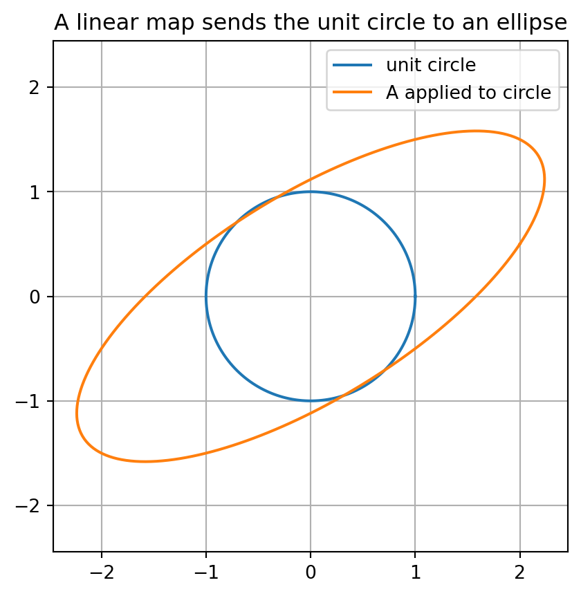
Let $A\in\mathbb R^{2\times2}$ be invertible. Then the image of the unit circle under $A$ is an ellipse. The lengths of the semi-major and semi-minor axes are the singular values of $A$.
:::
<details>
<summary>Proof</summary>
Let $A=U\Sigma V^T$, where
$$
\Sigma=\begin{bmatrix}\sigma_1&0\\0&\sigma_2\end{bmatrix},
\qquad
\sigma_1\ge\sigma_2>0.
$$
The map $V^T$ preserves the unit circle because it is orthogonal. The diagonal map $\Sigma$ sends the unit circle to the ellipse
$$
\frac{y_1^2}{\sigma_1^2}+\frac{y_2^2}{\sigma_2^2}=1.
$$
The map $U$ rotates or reflects this ellipse without changing its axis lengths. Therefore the semi-axis lengths are $\sigma_1$ and $\sigma_2$.
</details>
```{python}
import numpy as np
import matplotlib.pyplot as plt

A = np.array([[2.0, 1.0],
              [0.5, 1.5]])

t = np.linspace(0, 2*np.pi, 400)
circle = np.vstack([np.cos(t), np.sin(t)])
ellipse = A @ circle

plt.figure(figsize=(5,5))
plt.plot(circle[0], circle[1], label="unit circle")
plt.plot(ellipse[0], ellipse[1], label="A applied to circle")
plt.axis("equal")
plt.grid(True)
plt.legend()
plt.title("A linear map sends the unit circle to an ellipse")
plt.show()

print("Singular values:", np.linalg.svd(A, compute_uv=False))
```
## 14.8 Matrix norms and singular values
::: {.callout-note}
## Definition 14.9: Induced matrix norm
For a vector norm $\|\cdot\|_p$, the induced matrix norm is
$$
\|A\|_p
=\max_{x\ne0}\frac{\|Ax\|_p}{\|x\|_p}
=\max_{\|x\|_p=1}\|Ax\|_p.
$$
:::
::: {.callout-important}
## Theorem 14.10: Spectral norm
For every matrix $A$, the induced $2$-norm is the largest singular value:
$$
\|A\|_2=\sigma_1(A).
$$
:::
<details>
<summary>Proof</summary>
Let $A=U\Sigma V^T$. Since $U$ and $V$ are orthogonal, they preserve Euclidean norms. Thus
$$
\|Ax\|_2=\|U\Sigma V^Tx\|_2=\|\Sigma V^Tx\|_2.
$$
Let $y=V^Tx$. Then $\|y\|_2=\|x\|_2$. If $\|y\|_2=1$, then
$$
\|\Sigma y\|_2^2
=\sum_i \sigma_i^2y_i^2
\le \sigma_1^2\sum_i y_i^2
=\sigma_1^2.
$$
Therefore $\|A\|_2\le \sigma_1$. Equality is achieved when $y=e_1$, equivalently $x=v_1$. Hence $\|A\|_2=\sigma_1$.
</details>
## 14.9 The Moore--Penrose pseudoinverse
An invertible square matrix has an inverse. But rectangular or singular matrices usually do not. The SVD gives a replacement: the pseudoinverse.
::: {.callout-note}
## Definition 14.11: Moore--Penrose pseudoinverse
Let $A\in\mathbb R^{m\times n}$. A matrix $A^+\in\mathbb R^{n\times m}$ is called the **Moore--Penrose pseudoinverse** of $A$ if it satisfies
$$
AA^+A=A,
\qquad
A^+AA^+=A^+,
$$
$$
(AA^+)^T=AA^+,
\qquad
(A^+A)^T=A^+A.
$$
:::
::: {.callout-important}
## Theorem 14.12: Pseudoinverse from SVD
Let
$$
A=U\Sigma V^T
$$
be an SVD of $A$. Define $\Sigma^+$ by replacing each nonzero singular value $\sigma_i$ by $1/\sigma_i$ and transposing the rectangular diagonal shape. Then
$$
A^+=V\Sigma^+U^T.
$$
:::
```{python}
A = np.array([[1, 1],
              [1, 2],
              [1, 3]], dtype=float)
b = np.array([1, 2, 2], dtype=float)

x_pinv = np.linalg.pinv(A) @ b
x_lstsq, residuals, rank, s = np.linalg.lstsq(A, b, rcond=None)

print("Pseudoinverse solution:", x_pinv)
print("lstsq solution:", x_lstsq)
print("Residual norm:", np.linalg.norm(A @ x_pinv - b))
```
::: {.callout-important}
## Theorem 14.13: Least-squares and minimum-norm solution
For $A\in\mathbb R^{m\times n}$ and $b\in\mathbb R^m$, the vector
$$
x^+=A^+b
$$
is a least-squares solution of $Ax=b$. Among all least-squares solutions, it has minimum Euclidean norm.
:::
<details>
<summary>Proof</summary>
Write $A=U\Sigma V^T$, $y=V^Tx$, and $c=U^Tb$. Orthogonal transformations preserve Euclidean lengths, so
$$
\|Ax-b\|_2=\|U\Sigma V^Tx-b\|_2=\|\Sigma y-c\|_2.
$$
This is a diagonal least-squares problem. For each nonzero singular value, the best choice is
$$
y_i=\frac{c_i}{\sigma_i}.
$$
For zero singular values, the residual does not depend on $y_i$, so the minimum-norm choice is $y_i=0$. Transforming back gives
$$
x=V\Sigma^+U^Tb=A^+b.
$$
</details>
## 14.10 Low-rank approximation and compression
The SVD orders information by singular value size. Large singular values represent strong directions; small singular values represent weaker directions. This makes SVD ideal for compression.
::: {.callout-important}
## Theorem 14.14: Eckart--Young theorem
Let
$$
A=\sigma_1u_1v_1^T+\cdots+\sigma_pu_pv_p^T
$$
be the SVD of $A$, with $\sigma_1\ge\cdots\ge\sigma_p>0$. For $k<p$, define
$$
A_k=\sigma_1u_1v_1^T+\cdots+\sigma_ku_kv_k^T.
$$
Then $A_k$ is a best rank-$k$ approximation to $A$ in the spectral norm:
$$
\min_{\operatorname{rank}(B)\le k}\|A-B\|_2
=\|A-A_k\|_2
=\sigma_{k+1}.
$$
It is also best in the Frobenius norm:
$$
\min_{\operatorname{rank}(B)\le k}\|A-B\|_F
=\left(\sum_{i=k+1}^p\sigma_i^2\right)^{1/2}.
$$
:::
<details>
<summary>Proof idea</summary>
Orthogonal transformations preserve spectral and Frobenius norms. Therefore the approximation problem can be transformed into the problem of approximating the diagonal matrix $\Sigma$. The best rank-$k$ approximation keeps the largest $k$ diagonal entries and discards the rest. Transforming back gives $A_k$.
</details>
```{python}
# A small synthetic image-like matrix
x = np.linspace(-3, 3, 80)
y = np.linspace(-3, 3, 80)
Xgrid, Ygrid = np.meshgrid(x, y)
Image = np.exp(-(Xgrid**2 + Ygrid**2)) + 0.5*np.exp(-((Xgrid-1.2)**2 + (Ygrid+0.7)**2)/0.4)

U, s, Vt = np.linalg.svd(Image, full_matrices=False)

def rank_k(k):
    return U[:, :k] @ np.diag(s[:k]) @ Vt[:k, :]

for k in [1, 5, 10, 20]:
    Ak = rank_k(k)
    rel_error = np.linalg.norm(Image - Ak, 'fro') / np.linalg.norm(Image, 'fro')
    print(f"k={k:2d}, relative Frobenius error={rel_error:.4f}")
```
## 14.11 Principal component analysis
Suppose $X\in\mathbb R^{N\times d}$ is a data matrix whose rows are observations and whose columns are centered features. Then
$$
\frac{1}{N-1}X^TX
$$
is the sample covariance matrix. The right singular vectors of $X$ are the principal component directions.
::: {.callout-important}
## Proposition 14.15: PCA directions from SVD
The first principal component direction is the first right singular vector $v_1$ of $X$. More generally, the first $k$ principal directions are
$$
v_1,\ldots,v_k.
$$
The corresponding variances are proportional to
$$
\sigma_1^2,\ldots,\sigma_k^2.
$$
:::
<details>
<summary>Proof</summary>
PCA seeks a unit vector $v$ maximizing the variance of projected data:
$$
\|Xv\|_2^2=v^TX^TXv,
\qquad \|v\|_2=1.
$$
By the Rayleigh quotient theorem, the maximum is the largest eigenvalue of $X^TX$, achieved at its corresponding unit eigenvector. This is exactly the first right singular vector $v_1$, and the maximum value is $\lambda_1=\sigma_1^2$.
</details>
```{python}
np.random.seed(0)
Z = np.random.randn(200, 2)
Xdata = Z @ np.array([[3, 1], [0, 0.5]])
Xcentered = Xdata - Xdata.mean(axis=0)

U, s, Vt = np.linalg.svd(Xcentered, full_matrices=False)
print("Principal directions as rows of V^T:")
print(Vt)
print("Explained variance proportions:")
print(s**2 / np.sum(s**2))
```
## 14.12 Complex SVD
Over complex vector spaces, transpose is replaced by conjugate transpose.
::: {.callout-important}
## Theorem 14.16: Complex SVD
For every matrix $A\in\mathbb C^{m\times n}$, there exist unitary matrices
$$
U\in\mathbb C^{m\times m},
\qquad
V\in\mathbb C^{n\times n},
$$
and a rectangular diagonal matrix $\Sigma\in\mathbb R^{m\times n}$ with nonnegative diagonal entries such that
$$
A=U\Sigma V^*.
$$
The diagonal entries of $\Sigma$ are the square roots of the eigenvalues of the Hermitian positive semidefinite matrix $A^*A$.
:::
<details>
<summary>Proof</summary>
The matrix $A^*A$ is Hermitian because
$$
(A^*A)^*=A^*A.
$$
It is positive semidefinite because
$$
z^*A^*Az=\|Az\|_2^2\ge0.
$$
By the complex spectral theorem, there is a unitary matrix $V$ such that
$$
A^*A=VDV^*.
$$
Let $\sigma_i=\sqrt{\lambda_i}$. For positive $\sigma_i$, define
$$
u_i=\frac{Av_i}{\sigma_i}.
$$
The same orthogonality calculation shows these $u_i$ are orthonormal. Complete them to a unitary basis. Then $AV=U\Sigma$, so $A=U\Sigma V^*$.
</details>
## 14.13 Challenge questions
::: {.callout-question}
## Challenge 1
Why are singular values always nonnegative, even though eigenvalues can be negative?
:::
<details>
<summary>Solution</summary>
Singular values are square roots of eigenvalues of $A^TA$ or $A^*A$. These Gram matrices are positive semidefinite, so their eigenvalues are nonnegative. Therefore the singular values are nonnegative.
</details>
::: {.callout-question}
## Challenge 2
Explain why SVD exists for every matrix, while ordinary diagonalization does not.
:::
<details>
<summary>Solution</summary>
Ordinary diagonalization requires a square matrix with enough linearly independent eigenvectors. Many square matrices are defective, and rectangular matrices do not have ordinary eigenvalue decompositions. SVD applies the spectral theorem to $A^TA$ or $A^*A$, which is always symmetric or Hermitian positive semidefinite. Therefore SVD exists for every matrix.
</details>
::: {.callout-question}
## Challenge 3
Suppose the singular values of a matrix are $20,5,1,0.1$. What is the spectral norm error of the best rank-$2$ approximation?
:::
<details>
<summary>Solution</summary>
By Eckart--Young, the best rank-$2$ approximation error in spectral norm is the next singular value:
$$
\|A-A_2\|_2=\sigma_3=1.
$$
</details>
::: {.callout-question}
## Challenge 4
Suppose $A\in\mathbb R^{2\times2}$ has singular values $8$ and $1$. Describe the image of the unit circle under $A$.
:::
<details>
<summary>Solution</summary>
The image is an ellipse. Its semi-major axis has length $8$ and its semi-minor axis has length $1$. The directions of the axes are the left singular vectors.
</details>
## 14.14 Practice problems
::: {.callout-tip}
## Practice Problem 1
Let
$$
A=\begin{bmatrix}3&0\\0&2\end{bmatrix}.
$$
Find the singular values and describe the image of the unit circle.
:::
<details>
<summary>Solution</summary>
Since $A^TA=\operatorname{diag}(9,4)$, the singular values are $3$ and $2$. The unit circle is sent to the ellipse
$$
\frac{x^2}{9}+\frac{y^2}{4}=1.
$$
</details>
::: {.callout-tip}
## Practice Problem 2
Let
$$
A=\begin{bmatrix}1&1\\1&1\end{bmatrix}.
$$
Find the rank from the singular values.
:::
<details>
<summary>Solution</summary>
Compute
$$
A^TA=\begin{bmatrix}2&2\\2&2\end{bmatrix}.
$$
Its eigenvalues are $4$ and $0$. Therefore the singular values are $2$ and $0$. The rank is $1$.
</details>
::: {.callout-tip}
## Practice Problem 3
If a matrix has singular values $7,3,0,0$, what is its rank? What is its spectral norm?
:::
<details>
<summary>Solution</summary>
The rank is the number of nonzero singular values, so the rank is $2$. The spectral norm is the largest singular value, so $\|A\|_2=7$.
</details>
::: {.callout-tip}
## Practice Problem 4
Use Python to compute the SVD of
$$
A=\begin{bmatrix}1&4\\2&2\\2&-4\end{bmatrix}.
$$
Compare the singular values with the hand computation in the notes.
:::
<details>
<summary>Solution</summary>
```{python}
A = np.array([[1, 4], [2, 2], [2, -4]], dtype=float)
U, s, Vt = np.linalg.svd(A, full_matrices=True)
print(s)
```
The singular values are $6$ and $3$.
</details>
## 14.15 AI companion activities
Use an AI assistant as a study partner, not as a replacement for your own computation.
1. **Explain the story.** Ask: “Explain why SVD is a spectral theorem for rectangular matrices in three levels: beginner, applied math student, and data scientist.”
2. **Check a proof.** Ask the AI to verify the proof that $\ker(X^TX)=\ker(X)$, then identify the single most important line.
3. **Compare methods.** Ask: “Compare eigenvalue decomposition, Schur decomposition, and singular value decomposition.”
4. **Debug code.** Paste your SVD code and ask the AI to check dimensions of $U$, $\Sigma$, and $V^T$.
5. **Explore applications.** Ask for three examples where SVD appears in machine learning, image processing, or recommendation systems.
## 14.16 Summary
The singular value decomposition is one of the central tools of applied linear algebra:
$$
A=U\Sigma V^T
\qquad \text{or} \qquad
A=U\Sigma V^* \text{ over } \mathbb C.
$$
It generalizes the spectral theorem to all matrices. It explains geometry, rank, matrix norms, least squares, pseudoinverses, low-rank approximation, compression, and PCA. In modern applied mathematics, data science, and machine learning, SVD is not only a theorem; it is a computational language for extracting structure from data.