---
title: "Chapter TDA: Topological Data Analysis from Linear Algebra"
subtitle: "Turning shape into matrices"
author: "He Wang"
format:
html:
toc: true
number-sections: true
code-fold: true
code-tools: true
execute:
echo: true
warning: false
message: false
jupyter: python3
---
# The story: shape becomes linear algebra
A point cloud can look like a cloud of dots. A graph can look like a collection of edges. A triangle can look like a small drawing. Topological data analysis asks a more persistent question:
::: {.callout-important}
## Guiding question
What large-scale shape is hidden inside the data?
:::
In this chapter, we study topological data analysis from the point of view of applied linear algebra. The key message is simple and powerful:
::: {.callout-note}
## Main idea
Topological data analysis converts geometry into matrices. Then kernels, images, ranks, and quotient spaces detect connected components, loops, and higher-dimensional holes.
:::
The pipeline is
$$
\text{data}\longrightarrow \text{simplicial complex}\longrightarrow \text{boundary matrices}\longrightarrow \text{homology}\longrightarrow \text{features}.
$$
This chapter is not a full course in algebraic topology. Instead, it is a linear-algebra first introduction. We will see that the same tools used for null spaces and column spaces also compute Betti numbers and persistent homology.
# From data to shape
Classical clustering often asks how many connected components are present. TDA keeps this question but also asks whether the data contains loops, cavities, tunnels, or other holes.
::: {.callout-definition}
## Definition 1: Topological data analysis
**Topological data analysis** is a collection of methods that uses topological constructions and invariants to study data. A common workflow is:
1. start with data, often a point cloud $X\subseteq \mathbb R^d$;
2. build a simplicial complex from the data;
3. convert the complex into boundary matrices;
4. compute homology using linear algebra;
5. track homology across scales using persistent homology.
:::
The most basic topological summaries are the Betti numbers:
$$
\beta_0,\beta_1,\beta_2,\ldots.
$$
Their informal meanings are:
$$
\beta_0=\text{number of connected components},
$$
$$
\beta_1=\text{number of independent loops},
$$
$$
\beta_2=\text{number of independent enclosed voids}.
$$
# Simplices and simplicial complexes
Before building matrices, we need a combinatorial object that records points, edges, triangles, and higher-dimensional faces.
::: {.callout-definition}
## Definition 2: Simplex
A **$k$-simplex** is the convex hull of $k+1$ affinely independent points. These points are called vertices.
- A $0$-simplex is a vertex.
- A $1$-simplex is an edge.
- A $2$-simplex is a filled triangle.
- A $3$-simplex is a filled tetrahedron.
If the vertices are $v_0,v_1,\ldots,v_k$, the simplex is denoted by
$$
[v_0,v_1,\ldots,v_k].
$$
:::
::: {.callout-definition}
## Definition 3: Abstract simplicial complex
An **abstract simplicial complex** $K$ on a finite vertex set $V$ is a collection of finite subsets of $V$ such that if $\sigma\in K$ and $\tau\subseteq \sigma$, then $\tau\in K$.
Elements of $K$ are called **simplices**.
:::
The condition says that every face of a simplex must also be included. For example, if $[1,2,3]$ is in $K$, then the edges
$$
[1,2],\quad [1,3],\quad [2,3]
$$
and the vertices
$$
[1],\quad [2],\quad [3]
$$
must also be in $K$.
::: {.callout-example}
## Example 4: A small complex
Let $K$ have vertices $1,2,3,4$ and edges
$$
[1,2], [1,3], [2,3], [2,4], [3,4].
$$
Suppose that $[2,3,4]$ is a filled triangle but $[1,2,3]$ is not filled. Then the right triangle is filled, while the left triangle remains an open loop.
:::
# Chain spaces: replacing simplices by basis vectors
The first linear algebra step is to replace each simplex by a basis vector.
::: {.callout-definition}
## Definition 5: Chain space
Let $K$ be a finite simplicial complex and let $\mathbb F$ be a field, such as $\mathbb R$, $\mathbb Q$, or $\mathbb F_2$. The **$p$-chain space** $C_p(K;\mathbb F)$ is the vector space with basis given by the oriented $p$-simplices of $K$:
$$
C_p(K;\mathbb F)=\operatorname{span}_{\mathbb F}\{\text{oriented }p\text{-simplices of }K\}.
$$
A $p$-chain is a linear combination
$$
c=\sum_i a_i\sigma_i,
$$
where $a_i\in\mathbb F$ and $\sigma_i$ are $p$-simplices.
:::
If $K$ has $n_p$ simplices of dimension $p$, then
$$
C_p(K;\mathbb F)\cong \mathbb F^{n_p}.
$$
Thus a chain is just a coordinate vector once we choose an ordered basis of simplices.
::: {.callout-example}
## Example 6: Triangle boundary
Let $K$ be the boundary of a triangle with vertices $1,2,3$, but without the filled face. Then
$$
C_0=\operatorname{span}\{[1],[2],[3]\}\cong \mathbb F^3,
$$
$$
C_1=\operatorname{span}\{[1,2],[1,3],[2,3]\}\cong \mathbb F^3,
$$
and
$$
C_2=0.
$$
:::
# Boundary maps as matrices
A boundary map takes a simplex and returns its oriented boundary.
::: {.callout-definition}
## Definition 7: Boundary of a simplex
For an oriented $p$-simplex $[v_0,v_1,\ldots,v_p]$, define
$$
\partial_p[v_0,v_1,\ldots,v_p]
=
\sum_{i=0}^{p}(-1)^i[v_0,\ldots,\widehat{v_i},\ldots,v_p],
$$
where $\widehat{v_i}$ means that the vertex $v_i$ is omitted.
:::
The most important special cases are
$$
\partial_1[v_i,v_j]=[v_j]-[v_i],
$$
and
$$
\partial_2[v_i,v_j,v_k]=[v_j,v_k]-[v_i,v_k]+[v_i,v_j].
$$
::: {.callout-example}
## Example 8: Boundary matrix for a triangle boundary
Choose ordered bases
$$
C_1:([1,2],[1,3],[2,3]),
\qquad
C_0:([1],[2],[3]).
$$
Then
$$
\partial_1[1,2]=[2]-[1],
$$
$$
\partial_1[1,3]=[3]-[1],
$$
$$
\partial_1[2,3]=[3]-[2].
$$
Therefore
$$
[\partial_1]
=
\begin{bmatrix}
-1&-1&0\\
1&0&-1\\
0&1&1
\end{bmatrix}.
$$
Each column is the coordinate vector of the boundary of one edge.
:::
::: {.callout-example}
## Example 9: Boundary matrix for a filled triangle
Choose
$$
C_2:([1,2,3]),
\qquad
C_1:([1,2],[1,3],[2,3]).
$$
Since
$$
\partial_2[1,2,3]=[2,3]-[1,3]+[1,2],
$$
we have
$$
[\partial_2]=
\begin{bmatrix}
1\\-1\\1
\end{bmatrix}.
$$
:::
::: {.callout-theorem}
## Theorem 10: Boundary of a boundary is zero
For every $p\ge 1$,
$$
\partial_{p-1}\partial_p=0.
$$
Equivalently, in matrix form,
$$
[\partial_{p-1}][\partial_p]=0.
$$
:::
::: {.callout-tip collapse="true"}
## Proof of Theorem 10
It is enough to check the formula on a basis simplex $[v_0,\ldots,v_p]$. Applying $\partial_p$ deletes one vertex. Applying $\partial_{p-1}$ again deletes a second vertex. Every codimension-two face appears exactly twice: once by deleting $v_i$ first and $v_j$ second, and once by deleting $v_j$ first and $v_i$ second. The two signs are opposite, so the terms cancel. Therefore the total sum is zero.
:::
# Chain complexes, cycles, boundaries, and homology
The boundary maps fit together into a chain complex.
::: {.callout-definition}
## Definition 11: Chain complex
A **chain complex** is a sequence of vector spaces and linear maps
$$
\cdots\longrightarrow C_{p+1}\xrightarrow{\partial_{p+1}}C_p\xrightarrow{\partial_p}C_{p-1}\xrightarrow{\partial_{p-1}}\cdots
$$
such that
$$
\partial_p\partial_{p+1}=0
$$
for all $p$.
:::
::: {.callout-definition}
## Definition 12: Cycles and boundaries
The space of **$p$-cycles** is
$$
Z_p=\ker(\partial_p),
$$
and the space of **$p$-boundaries** is
$$
B_p=\operatorname{im}(\partial_{p+1}).
$$
:::
Cycles are chains with no boundary. Boundaries are chains that are already boundaries of higher-dimensional chains.
::: {.callout-proposition}
## Proposition 13: Boundaries are cycles
For every $p$,
$$
B_p\subseteq Z_p.
$$
:::
::: {.callout-tip collapse="true"}
## Proof of Proposition 13
If $\vec x\in B_p$, then $\vec x=\partial_{p+1}\vec y$ for some $\vec y\in C_{p+1}$. Therefore
$$
\partial_p\vec x=\partial_p\partial_{p+1}\vec y=0.
$$
Thus $\vec x\in\ker(\partial_p)=Z_p$.
:::
::: {.callout-definition}
## Definition 14: Homology and Betti numbers
The **$p$-th homology vector space** is
$$
H_p=Z_p/B_p
=
\ker(\partial_p)/\operatorname{im}(\partial_{p+1}).
$$
The **$p$-th Betti number** is
$$
\beta_p=\dim H_p.
$$
:::
The quotient is the key idea. We count cycles, but we do not count cycles that are already boundaries.
::: {.callout-theorem}
## Theorem 15: Betti numbers from ranks
For a finite chain complex over a field,
$$
\beta_p
=
\dim\ker(\partial_p)-\operatorname{rank}(\partial_{p+1}).
$$
Equivalently,
$$
\boxed{\beta_p=\dim C_p-\operatorname{rank}(\partial_p)-\operatorname{rank}(\partial_{p+1}).}
$$
:::
::: {.callout-tip collapse="true"}
## Proof of Theorem 15
Since $B_p\subseteq Z_p$ and both are finite-dimensional vector spaces,
$$
\dim(Z_p/B_p)=\dim Z_p-\dim B_p.
$$
Now $Z_p=\ker(\partial_p)$ and $B_p=\operatorname{im}(\partial_{p+1})$, so
$$
\beta_p=\dim\ker(\partial_p)-\operatorname{rank}(\partial_{p+1}).
$$
By rank-nullity,
$$
\dim\ker(\partial_p)=\dim C_p-\operatorname{rank}(\partial_p).
$$
Substituting gives
$$
\beta_p=\dim C_p-\operatorname{rank}(\partial_p)-\operatorname{rank}(\partial_{p+1}).
$$
:::
# Worked examples
## Example 16: One edge and one isolated vertex
Let
$$
K=\{[1],[2],[3],[1,2]\}.
$$
This is one edge together with one isolated vertex. Choose bases
$$
C_1:([1,2]),
\qquad
C_0:([1],[2],[3]).
$$
Then
$$
[\partial_1]=
\begin{bmatrix}
-1\\1\\0
\end{bmatrix}.
$$
So $\operatorname{rank}(\partial_1)=1$, $\partial_0=0$, and $\partial_2=0$. Therefore
$$
\beta_0=\dim C_0-\operatorname{rank}(\partial_0)-\operatorname{rank}(\partial_1)=3-0-1=2,
$$
and
$$
\beta_1=\dim C_1-\operatorname{rank}(\partial_1)-\operatorname{rank}(\partial_2)=1-1-0=0.
$$
The complex has two connected components and no loop.
## Example 17: A triangle boundary
Let $K$ be the triangle boundary with vertices $1,2,3$ and no filled face. Then
$$
[\partial_1]=
\begin{bmatrix}
-1&-1&0\\
1&0&-1\\
0&1&1
\end{bmatrix}.
$$
The graph is connected, so $\operatorname{rank}(\partial_1)=2$. Since there is no $2$-simplex, $\partial_2=0$. Thus
$$
\beta_0=3-0-2=1,
$$
and
$$
\beta_1=3-2-0=1.
$$
There is one connected component and one loop.
## Example 18: A filled triangle
Now include the face $[1,2,3]$. The matrix $\partial_1$ is the same, but
$$
[\partial_2]=
\begin{bmatrix}
1\\-1\\1
\end{bmatrix}.
$$
Thus $\operatorname{rank}(\partial_1)=2$ and $\operatorname{rank}(\partial_2)=1$. Hence
$$
\beta_0=3-0-2=1,
$$
$$
\beta_1=3-2-1=0,
$$
and
$$
\beta_2=1-1-0=0.
$$
Filling the triangle kills the one-dimensional hole.
## Example 19: Two triangles, one filled
Consider vertices $1,2,3,4$, edges
$$
[1,2], [1,3], [2,3], [2,4], [3,4],
$$
and one filled face $[2,3,4]$. Choose bases
$$
C_0:([1],[2],[3],[4]),
$$
$$
C_1:([1,2],[1,3],[2,3],[2,4],[3,4]),
$$
$$
C_2:([2,3,4]).
$$
Then
$$
[\partial_1]=
\begin{bmatrix}
-1&-1&0&0&0\\
1&0&-1&-1&0\\
0&1&1&0&-1\\
0&0&0&1&1
\end{bmatrix},
$$
and
$$
[\partial_2]=
\begin{bmatrix}
0\\0\\1\\-1\\1
\end{bmatrix}.
$$
The complex is connected, so $\operatorname{rank}(\partial_1)=3$. Also $\operatorname{rank}(\partial_2)=1$. Therefore
$$
\beta_0=4-0-3=1,
$$
$$
\beta_1=5-3-1=1,
$$
and
$$
\beta_2=1-1-0=0.
$$
There is one remaining loop: the unfilled triangle $[1,2,3]$.
# Python computation: Betti numbers from boundary matrices
The formulas above are easy to compute once the boundary matrices are known.
```{python}
import numpy as np


def rank(A, tol=1e-10):
    """Numerical matrix rank."""
    A = np.array(A, dtype=float)
    if A.size == 0:
        return 0
    return np.linalg.matrix_rank(A, tol=tol)


def betti(dim_Cp, boundary_p, boundary_p_plus_1):
    """
    beta_p = dim C_p - rank(partial_p) - rank(partial_{p+1}).
    """
    return dim_Cp - rank(boundary_p) - rank(boundary_p_plus_1)

# Triangle boundary
partial1 = np.array([
    [-1, -1,  0],
    [ 1,  0, -1],
    [ 0,  1,  1]
], dtype=float)
partial2_empty = np.zeros((3, 0))
partial0 = np.zeros((0, 3))

beta0 = betti(3, partial0, partial1)
beta1 = betti(3, partial1, partial2_empty)
print("Triangle boundary: beta0, beta1 =", beta0, beta1)

# Filled triangle
partial2_filled = np.array([[1], [-1], [1]], dtype=float)
beta1_filled = betti(3, partial1, partial2_filled)
print("Filled triangle: beta1 =", beta1_filled)
```
# Constructing boundary matrices automatically
We can generate boundary matrices from lists of simplices.
```{python}
from itertools import combinations


def simplex_faces(simplex):
    """Oriented codimension-one faces of a simplex."""
    simplex = tuple(simplex)
    faces = []
    for i in range(len(simplex)):
        face = simplex[:i] + simplex[i+1:]
        sign = (-1)**i
        faces.append((face, sign))
    return faces


def boundary_matrix(p_simplices, pm1_simplices):
    """Boundary matrix from p-simplices to (p-1)-simplices over R."""
    row_index = {s:i for i,s in enumerate(pm1_simplices)}
    M = np.zeros((len(pm1_simplices), len(p_simplices)))
    for j, sigma in enumerate(p_simplices):
        for face, sign in simplex_faces(sigma):
            M[row_index[face], j] = sign
    return M

vertices = [(1,), (2,), (3,), (4,)]
edges = [(1,2), (1,3), (2,3), (2,4), (3,4)]
faces = [(2,3,4)]

D1 = boundary_matrix(edges, vertices)
D2 = boundary_matrix(faces, edges)

print("D1 =")
print(D1.astype(int))
print("D2 =")
print(D2.astype(int))
print("beta0 =", betti(len(vertices), np.zeros((0,len(vertices))), D1))
print("beta1 =", betti(len(edges), D1, D2))
print("beta2 =", betti(len(faces), D2, np.zeros((0,len(faces)))))
```
# Building complexes from data
In applications, we often start from a point cloud
$$
X=\{\vec x_1,\ldots,\vec x_N\}\subseteq \mathbb R^d.
$$
We then build a simplicial complex using pairwise distances.
::: {.callout-definition}
## Definition 20: Vietoris--Rips complex
Let $X$ be a finite metric space and let $r\ge 0$. The **Vietoris--Rips complex** $\operatorname{VR}_r(X)$ is the simplicial complex whose vertices are the points of $X$, and whose $k$-simplices are subsets
$$
\{x_{i_0},\ldots,x_{i_k}\}
$$
such that
$$
d(x_{i_a},x_{i_b})\le r
$$
for all pairs $a,b$.
:::
Equivalently, $\operatorname{VR}_r(X)$ is the clique complex of the graph that connects two points when their distance is at most $r$.
::: {.callout-example}
## Example 21: Six points on a circle
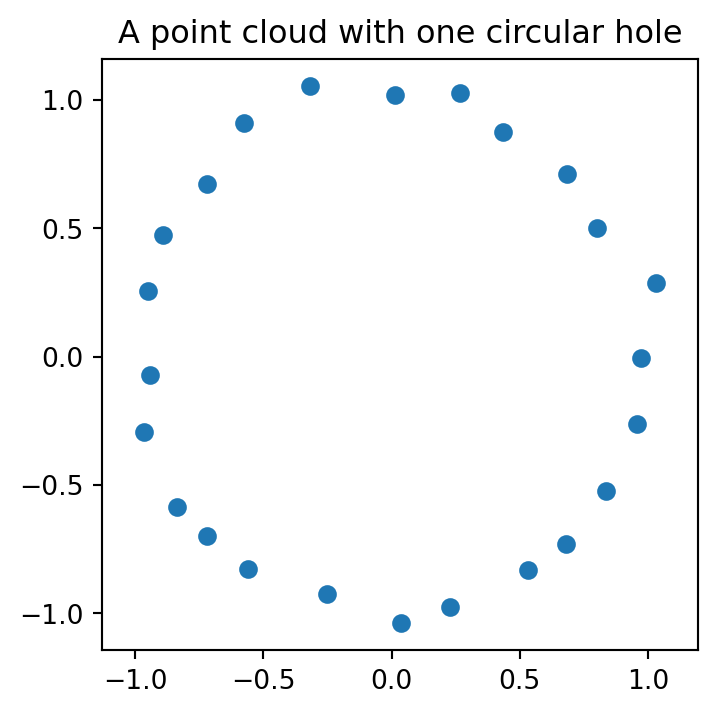
If six points lie approximately on a circle, then for a suitable scale $r$, the Vietoris--Rips complex may contain edges forming a loop but not enough filled triangles to fill the loop. At that scale, $\beta_1=1$.
:::
```{python}
import matplotlib.pyplot as plt

# Points on a noisy circle
rng = np.random.default_rng(4)
theta = np.linspace(0, 2*np.pi, 24, endpoint=False)
X = np.c_[np.cos(theta), np.sin(theta)] + 0.04*rng.normal(size=(24,2))

plt.figure(figsize=(4,4))
plt.scatter(X[:,0], X[:,1])
plt.axis("equal")
plt.title("A point cloud with one circular hole")
plt.show()
```
# Filtrations and persistent homology
A single scale can be misleading. If $r$ is too small, the complex is disconnected. If $r$ is too large, everything may become filled in. Persistent homology studies all scales together.
::: {.callout-definition}
## Definition 22: Filtration
A **filtration** is a nested sequence of simplicial complexes
$$
K_0\subseteq K_1\subseteq K_2\subseteq \cdots\subseteq K_m.
$$
For a point cloud, a common filtration is
$$
\operatorname{VR}_{r_0}(X)\subseteq \operatorname{VR}_{r_1}(X)\subseteq\cdots\subseteq\operatorname{VR}_{r_m}(X),
$$
where
$$
0\le r_0\le r_1\le\cdots\le r_m.
$$
:::
::: {.callout-definition}
## Definition 23: Persistence barcode
A **persistence barcode** records the birth and death intervals of homology classes across a filtration. A bar
$$
[b,d)
$$
means that a homology class appears at filtration value $b$ and disappears at filtration value $d$.
:::
A long $H_0$ bar corresponds to a connected component that persists across many scales. A long $H_1$ bar corresponds to a loop that persists across many scales. Short bars are often interpreted as noise, although this depends on the data and application.
# Persistent homology as matrix reduction
Persistent homology also reduces to linear algebra.
::: {.callout-definition}
## Definition 24: Filtration order
A **filtration order** is an ordering of simplices
$$
\sigma_1,\sigma_2,\ldots,\sigma_N
$$
such that every face of a simplex appears before the simplex itself.
:::
::: {.callout-definition}
## Definition 25: Total boundary matrix
The **total boundary matrix** $D$ is the matrix whose $j$-th column is the boundary of $\sigma_j$ written in the ordered simplex basis $\sigma_1,\ldots,\sigma_N$.
:::
The standard persistence algorithm performs column operations on $D$, similar to Gaussian elimination. These operations reveal which simplices create homology classes and which simplices kill them.
::: {.callout-definition}
## Definition 26: Low index
For a nonzero column $j$ of a matrix $R$, define
$$
\operatorname{low}(j)=\max\{i:R_{ij}\neq 0\}.
$$
A matrix is **reduced** if no two nonzero columns have the same low index.
:::
::: {.callout-proposition}
## Proposition 27: Persistence pairing
In a reduced boundary matrix, if $\operatorname{low}(j)=i$, then simplex $\sigma_i$ creates a homology class and simplex $\sigma_j$ kills it. The corresponding persistence interval is
$$
[\operatorname{time}(\sigma_i),\operatorname{time}(\sigma_j)).
$$
Unpaired creating simplices give infinite bars.
:::
::: {.callout-note}
## Why this belongs in applied linear algebra
Persistence computation is structured Gaussian elimination over a field, often $\mathbb F_2$. The data object is a matrix, and the algorithm is a reduction algorithm.
:::
# Coefficients: real numbers or $\mathbb F_2$?
The field of coefficients affects the signs in boundary formulas.
- Over $\mathbb R$ or $\mathbb Q$, orientations and signs matter.
- Over $\mathbb F_2$, signs disappear because $-1=1$.
- Many computational TDA packages use $\mathbb F_2$ for speed and simplicity.
::: {.callout-example}
## Example 28: Boundary over $\mathbb F_2$
Over $\mathbb R$,
$$
\partial_2[1,2,3]=[2,3]-[1,3]+[1,2].
$$
Over $\mathbb F_2$,
$$
\partial_2[1,2,3]=[2,3]+[1,3]+[1,2].
$$
The chain-complex condition still holds:
$$
\partial_1\partial_2=0.
$$
:::
# TDA features for machine learning
After persistent homology is computed, the output can be converted into numerical features.
::: {.callout-definition}
## Definition 29: Persistence diagram
A **persistence diagram** is the multiset of points
$$
(b_i,d_i),
$$
where $b_i$ and $d_i$ are the birth and death times of homology classes.
:::
::: {.callout-definition}
## Definition 30: Persistence images and landscapes
**Persistence images** and **persistence landscapes** are vectorized summaries of persistence diagrams. They convert topological information into feature vectors for regression, classification, clustering, or deep learning.
:::
A typical machine-learning pipeline is
$$
\text{point cloud}
\longrightarrow
\text{filtration}
\longrightarrow
\text{boundary matrices}
\longrightarrow
\text{barcodes}
\longrightarrow
\text{feature vectors}
\longrightarrow
\text{ML model}.
$$
# Challenge questions
## Challenge 1: Why quotient spaces appear
In homology, why do we define
$$
H_p=Z_p/B_p
$$
instead of simply using $Z_p$?
::: {.callout-tip collapse="true"}
## Solution
Cycles include all closed objects, but some closed objects are boundaries of higher-dimensional objects. Boundaries should not count as holes. For example, the boundary of a filled triangle is a cycle, but it does not represent a one-dimensional hole because it bounds a $2$-simplex. The quotient
$$
Z_p/B_p
$$
identifies cycles that differ by a boundary. Thus homology keeps only cycles not explained as boundaries.
:::
## Challenge 2: One filled triangle and one open triangle
For the complex in Example 19, explain conceptually why $\beta_1=1$ without doing row reduction.
::: {.callout-tip collapse="true"}
## Solution
There are two triangular loops sharing an edge: the left loop $[1,2,3]$ and the right loop $[2,3,4]$. The right triangle is filled by a $2$-simplex, so its boundary is a boundary and does not count as a hole. The left triangle is not filled, so its loop remains. The complex is connected and has one independent unfilled loop. Hence $\beta_0=1$ and $\beta_1=1$.
:::
## Challenge 3: Rank-nullity interpretation
Suppose a finite complex has
$$
\dim C_2=4,
\qquad
\dim C_1=10,
\qquad
\dim C_0=7,
$$
with
$$
\operatorname{rank}(\partial_2)=3,
\qquad
\operatorname{rank}(\partial_1)=6.
$$
Assume $C_3=0$. Find $\beta_0,\beta_1,\beta_2$.
::: {.callout-tip collapse="true"}
## Solution
Using
$$
\beta_p=\dim C_p-\operatorname{rank}(\partial_p)-\operatorname{rank}(\partial_{p+1}),
$$
we get
$$
\beta_0=7-0-6=1,
$$
$$
\beta_1=10-6-3=1,
$$
and since $C_3=0$,
$$
\beta_2=4-3-0=1.
$$
Thus the complex has one connected component, one independent loop, and one independent two-dimensional void.
:::
## Challenge 4: Persistent versus non-persistent loops
Suppose a point cloud produces two $H_1$ bars:
$$
[0.18,0.22),
\qquad
[0.25,1.10).
$$
Which one is more likely to represent a meaningful loop in the data?
::: {.callout-tip collapse="true"}
## Solution
The bar $[0.25,1.10)$ is much longer. It persists across a larger range of scales, so it is more likely to represent a genuine geometric feature of the data. The short bar $[0.18,0.22)$ may be caused by sampling noise or a small accidental configuration of points. This is a useful heuristic, but interpretation still depends on the data and application.
:::
## Challenge 5: A matrix condition for no one-dimensional holes
Let $K$ be a connected two-dimensional simplicial complex. Give a rank condition involving $\partial_1$ and $\partial_2$ that implies $\beta_1=0$.
::: {.callout-tip collapse="true"}
## Solution
Since
$$
\beta_1=\dim C_1-\operatorname{rank}(\partial_1)-\operatorname{rank}(\partial_2),
$$
we have $\beta_1=0$ exactly when
$$
\operatorname{rank}(\partial_1)+\operatorname{rank}(\partial_2)=\dim C_1.
$$
Equivalently,
$$
\ker(\partial_1)=\operatorname{im}(\partial_2),
$$
meaning every $1$-cycle is the boundary of a $2$-chain.
:::
# Practice problems
## Problem 1
Let $K$ have vertices $1,2,3$ and one edge $[1,2]$. Compute $\beta_0$ and $\beta_1$.
::: {.callout-tip collapse="true"}
## Solution
There are two connected components: the edge component containing $1,2$, and the isolated vertex $3$. There are no loops. Thus
$$
\beta_0=2,
\qquad
\beta_1=0.
$$
:::
## Problem 2
For the triangle boundary without a filled face, write the boundary matrix $\partial_1$ using edge basis $([1,2],[1,3],[2,3])$ and vertex basis $([1],[2],[3])$.
::: {.callout-tip collapse="true"}
## Solution
The columns are
$$
\partial_1[1,2]=[2]-[1],
$$
$$
\partial_1[1,3]=[3]-[1],
$$
$$
\partial_1[2,3]=[3]-[2].
$$
Therefore
$$
[\partial_1]
=
\begin{bmatrix}
-1&-1&0\\
1&0&-1\\
0&1&1
\end{bmatrix}.
$$
:::
## Problem 3
For a filled triangle, explain why $\beta_1=0$.
::: {.callout-tip collapse="true"}
## Solution
The boundary of the triangle is a cycle, but it is the boundary of the filled $2$-simplex. Since boundaries are identified with zero in homology, the loop does not count as a hole. Therefore $\beta_1=0$.
:::
## Problem 4
A complex has $\dim C_0=8$, $\dim C_1=12$, $\dim C_2=5$, $\operatorname{rank}(\partial_1)=7$, and $\operatorname{rank}(\partial_2)=4$. Assume $C_3=0$. Compute $\beta_0,\beta_1,\beta_2$.
::: {.callout-tip collapse="true"}
## Solution
Using the rank formula,
$$
\beta_0=8-0-7=1,
$$
$$
\beta_1=12-7-4=1,
$$
and
$$
\beta_2=5-4-0=1.
$$
:::
## Problem 5
Explain why the Vietoris--Rips complex of a point cloud grows as the scale $r$ increases.
::: {.callout-tip collapse="true"}
## Solution
If $r_1\le r_2$, then any pair of points with distance at most $r_1$ also has distance at most $r_2$. Therefore every simplex in $\operatorname{VR}_{r_1}(X)$ is also a simplex in $\operatorname{VR}_{r_2}(X)$. Hence
$$
\operatorname{VR}_{r_1}(X)\subseteq \operatorname{VR}_{r_2}(X).
$$
:::
# AI companion activities
Use an AI assistant as a study companion, but verify every mathematical claim with definitions and computations.
::: {.callout-note}
## Activity 1: Explain the quotient
Ask:
> Explain why homology is $Z_p/B_p$ rather than just $Z_p$, using the filled triangle as an example.
Then check whether the answer correctly distinguishes cycles from boundaries.
:::
::: {.callout-note}
## Activity 2: Generate boundary matrices
Ask:
> Given vertices, edges, and filled triangles of a simplicial complex, write the boundary matrices $\partial_1$ and $\partial_2$.
Then verify the matrices by checking that each column is the boundary of one simplex.
:::
::: {.callout-note}
## Activity 3: Interpret barcodes
Ask:
> Given a barcode with several short bars and one long bar in $H_1$, explain which features might represent signal and which might represent noise.
Then ask what assumptions are being made.
:::
::: {.callout-note}
## Activity 4: Connect TDA to machine learning
Ask:
> How can persistence diagrams be converted into feature vectors for a machine-learning model?
Compare persistence images, landscapes, and simple summary statistics such as total persistence.
:::
# Summary
The central message of this chapter is that TDA is built from linear algebra:
- simplices become basis vectors;
- boundary maps become matrices;
- cycles become null spaces;
- boundaries become column spaces;
- homology becomes a quotient vector space;
- Betti numbers become rank-nullity computations;
- persistent homology becomes structured matrix reduction.
Thus TDA is not separate from applied linear algebra. It is one of the clearest examples of abstract linear algebra becoming a computational tool for modern data analysis.