---
title: "Chapter 16: Fast Fourier Transforms"
subtitle: "From Time Samples to Frequency Coordinates"
author: "He Wang"
format:
html:
toc: true
number-sections: true
code-fold: true
code-tools: true
jupyter: python3
---
# Chapter 16: Fast Fourier Transforms
## Opening story: hearing a vector as a chord
A sound wave looks like a long list of numbers when it is recorded by a microphone. Each number is a sample at one instant of time. In the standard basis, the signal is simply
$$
\vec f=\begin{bmatrix}f_0\\ f_1\\ \vdots\\ f_{n-1}\end{bmatrix}.
$$
But a musician does not usually hear a sound as a long list of samples. A musician hears pitch, rhythm, and resonance. In mathematical language, we want a new coordinate system that describes the same vector by its **frequencies**.
Fourier analysis is the linear algebra of this change of coordinates. The discrete Fourier transform changes a vector from the time/sample basis into a frequency basis. The fast Fourier transform, or FFT, is a fast algorithm for computing the same change of coordinates.
::: {.callout-note}
## Main idea
The discrete Fourier transform is multiplication by a special matrix $F_n$. The FFT is not a different transform and not an approximation. It is a faster way to compute $F_n\vec f$ by using the structure of roots of unity.
:::
## 1. Fourier methods as linear algebra
Fourier analysis is often introduced in differential equations or signal processing. In this course we view it as applied linear algebra:
$$
\text{data in time coordinates}
\quad\longrightarrow\quad
\text{data in frequency coordinates}.
$$
The same vector can be described in different bases. Earlier chapters used bases such as the standard basis, eigenvector bases, orthonormal bases, and Haar bases. Fourier methods use basis vectors made from complex waves.
The practical reason is powerful: in the Fourier basis, many operations become simpler.
- Oscillations separate into basic frequencies.
- Convolution becomes pointwise multiplication.
- Difference equations become algebraic equations.
- Circulant matrices become diagonal.
- Fast algorithms become possible.
::: {.callout-tip}
## Historical motivation
Joseph Fourier studied heat flow. A complicated temperature profile can be decomposed into simple heat modes. This is one of the earliest and most influential examples of changing basis to solve a problem.
:::
## 2. Hermitian inner products on functions
Fourier series begins with orthogonality of functions. For complex-valued functions $f,g:[a,b]\to\mathbb C$, the Hermitian inner product is
$$
\langle f,g\rangle=\int_a^b f(x)\overline{g(x)}\,dx.
$$
The complex conjugate is essential because it gives
$$
\langle f,f\rangle=\int_a^b |f(x)|^2\,dx\ge 0.
$$
::: {.callout-important}
## Definition 16.1: Orthogonality of functions
Two functions $f$ and $g$ are **orthogonal** on $[a,b]$ if
$$
\langle f,g\rangle=0.
$$
A family $\{\phi_k\}$ is orthogonal if $\langle \phi_j,\phi_k\rangle=0$ whenever $j\ne k$.
:::
### Example 16.2: Trigonometric orthogonality
On $[-\pi,\pi]$, the functions $\cos(kx)$ and $\sin(kx)$ satisfy
$$
\int_{-\pi}^{\pi}\cos(jx)\cos(kx)\,dx=0\qquad (j\ne k),
$$
$$
\int_{-\pi}^{\pi}\sin(jx)\sin(kx)\,dx=0\qquad (j\ne k),
$$
and
$$
\int_{-\pi}^{\pi}\cos(jx)\sin(kx)\,dx=0.
$$
This is the function-space version of orthogonal vectors in $\mathbb R^n$.
## 3. Fourier series as orthogonal projection
If $f$ is $2\pi$-periodic, its real Fourier series has the form
$$
f(x)\sim \frac{a_0}{2}+\sum_{k=1}^{\infty}\left(a_k\cos(kx)+b_k\sin(kx)\right),
$$
where
$$
a_k=\frac1\pi\int_{-\pi}^{\pi} f(x)\cos(kx)\,dx,
\qquad
b_k=\frac1\pi\int_{-\pi}^{\pi} f(x)\sin(kx)\,dx.
$$
These coefficients are projection coefficients. The finite Fourier approximation is the orthogonal projection of $f$ onto the finite-dimensional subspace spanned by
$$
1,\cos x,\sin x,\ldots,\cos(mx),\sin(mx).
$$
For an $L$-periodic function on $[0,L)$,
$$
f(x)\sim \frac{a_0}{2}+\sum_{k=1}^{\infty}\left(a_k\cos\frac{2\pi kx}{L}+b_k\sin\frac{2\pi kx}{L}\right),
$$
with
$$
a_k=\frac{2}{L}\int_0^L f(x)\cos\frac{2\pi kx}{L}\,dx,
\qquad
b_k=\frac{2}{L}\int_0^L f(x)\sin\frac{2\pi kx}{L}\,dx.
$$
## 4. Complex Fourier series
Euler's formula says
$$
e^{ix}=\cos x+i\sin x.
$$
Define
$$
\psi_k(x)=e^{ikx},\qquad k\in\mathbb Z.
$$
Then
$$
\langle \psi_j,\psi_k\rangle
=\int_{-\pi}^{\pi}e^{ijx}\overline{e^{ikx}}\,dx
=\int_{-\pi}^{\pi}e^{i(j-k)x}\,dx.
$$
::: {.callout-tip}
## Proposition 16.3: Orthogonality of complex exponentials
The functions $\psi_k(x)=e^{ikx}$ satisfy
$$
\langle \psi_j,\psi_k\rangle=
\begin{cases}
0, & j\ne k,\\
2\pi, & j=k.
\end{cases}
$$
:::
<details>
<summary><strong>Show proof</strong></summary>
If $j=k$, then
$$
\langle \psi_j,\psi_j\rangle=\int_{-\pi}^{\pi}1\,dx=2\pi.
$$
If $j\ne k$, then
$$
\int_{-\pi}^{\pi}e^{i(j-k)x}\,dx
=\left[\frac{e^{i(j-k)x}}{i(j-k)}\right]_{-\pi}^{\pi}=0,
$$
because $e^{i(j-k)\pi}=e^{-i(j-k)\pi}=(-1)^{j-k}$.
</details>
::: {.callout-important}
## Theorem 16.4: Complex Fourier coefficients
If $f$ is a suitable $2\pi$-periodic complex-valued function, then
$$
f(x)\sim \sum_{k=-\infty}^{\infty}c_ke^{ikx},
$$
where
$$
c_k=\frac{1}{2\pi}\int_{-\pi}^{\pi}f(x)e^{-ikx}\,dx
=\frac{\langle f,\psi_k\rangle}{\langle \psi_k,\psi_k\rangle}.
$$
:::
<details>
<summary><strong>Show proof</strong></summary>
This is the standard coordinate formula in an orthogonal basis. If
$$
f\approx \sum_k c_k\psi_k,
$$
then taking the inner product with $\psi_j$ gives
$$
\langle f,\psi_j\rangle\approx \sum_k c_k\langle \psi_k,\psi_j\rangle
=c_j\langle \psi_j,\psi_j\rangle.
$$
Since $\langle \psi_j,\psi_j\rangle=2\pi$, we obtain
$$
c_j=\frac{1}{2\pi}\langle f,\psi_j\rangle.
$$
</details>
## 5. The continuous Fourier transform
Fourier series is designed for periodic functions. For nonperiodic functions, we use the Fourier transform. With one common convention,
$$
\widehat f(\omega)=\mathcal F(f)(\omega)
=\int_{-\infty}^{\infty}f(x)e^{-i\omega x}\,dx.
$$
The inverse transform is
$$
f(x)=\mathcal F^{-1}(\widehat f)(x)
=\frac{1}{2\pi}\int_{-\infty}^{\infty}\widehat f(\omega)e^{i\omega x}\,d\omega.
$$
::: {.callout-note}
## Remark: Where the $2\pi$ goes
Different books place the $2\pi$ in different locations. Some use $e^{-2\pi i sx}$. Some split constants between the transform and inverse transform. The main ideas are unchanged, but constants differ.
:::
::: {.callout-tip}
## Proposition 16.5: Derivatives become multiplication
If $f$ decays sufficiently fast at infinity, then
$$
\mathcal F(f')(\omega)=i\omega\widehat f(\omega).
$$
:::
<details>
<summary><strong>Show proof</strong></summary>
Using integration by parts,
$$
\begin{aligned}
\mathcal F(f')(\omega)
&=\int_{-\infty}^{\infty}f'(x)e^{-i\omega x}\,dx\\
&=\left[f(x)e^{-i\omega x}\right]_{-\infty}^{\infty}
+i\omega\int_{-\infty}^{\infty}f(x)e^{-i\omega x}\,dx.
\end{aligned}
$$
The boundary term is zero under the decay assumption. Therefore
$$
\mathcal F(f')(\omega)=i\omega\widehat f(\omega).
$$
</details>
::: {.callout-important}
## Theorem 16.6: Parseval identity
For suitable functions,
$$
\int_{-\infty}^{\infty}|\widehat f(\omega)|^2\,d\omega
=2\pi\int_{-\infty}^{\infty}|f(x)|^2\,dx.
$$
Thus the Fourier transform preserves energy up to a constant depending on convention.
:::
## 6. From continuous signals to discrete data
Computers store finite vectors, not full functions. A sampled signal is
$$
\vec f=\begin{bmatrix}f_0\\ f_1\\ \vdots\\ f_{n-1}\end{bmatrix}\in\mathbb C^n.
$$
The discrete Fourier transform changes this vector from time coordinates to frequency coordinates.
::: {.callout-important}
## Definition 16.7: Discrete Fourier transform
Let
$$
\omega_n=e^{-2\pi i/n}.
$$
For $\vec f=(f_0,\ldots,f_{n-1})^T\in\mathbb C^n$, the **discrete Fourier transform** is the vector $\widehat{\vec f}\in\mathbb C^n$ defined by
$$
\widehat f_k=\sum_{j=0}^{n-1}f_j\omega_n^{jk},
\qquad k=0,1,\ldots,n-1.
$$
The inverse discrete Fourier transform is
$$
f_j=\frac1n\sum_{k=0}^{n-1}\widehat f_k\omega_n^{-jk},
\qquad j=0,1,\ldots,n-1.
$$
:::
::: {.callout-important}
## Definition 16.8: Fourier matrix
The Fourier matrix is
$$
F_n=\left[\omega_n^{jk}\right]_{j,k=0}^{n-1}.
$$
With this convention,
$$
\widehat{\vec f}=F_n\vec f.
$$
:::
### Example 16.9: The Fourier matrix for $n=4$
Since $\omega_4=e^{-2\pi i/4}=-i$,
$$
F_4=
\begin{bmatrix}
1&1&1&1\\
1&-i&-1&i\\
1&-1&1&-1\\
1&i&-1&-i
\end{bmatrix}.
$$
## 7. Roots of unity and orthogonality
The entries of the Fourier matrix are powers of roots of unity. The complex numbers satisfying $z^n=1$ are
$$
1,\omega_n,\omega_n^2,\ldots,\omega_n^{n-1}.
$$
They lie evenly spaced around the unit circle.
::: {.callout-tip}
## Lemma 16.10: Geometric sum identity
If $q\ne 1$ and $q^n=1$, then
$$
1+q+q^2+\cdots+q^{n-1}=0.
$$
:::
<details>
<summary><strong>Show proof</strong></summary>
Using the finite geometric sum formula,
$$
1+q+\cdots+q^{n-1}=\frac{1-q^n}{1-q}=\frac{1-1}{1-q}=0.
$$
</details>
::: {.callout-tip}
## Theorem 16.11: Orthogonality of the Fourier matrix
The columns of $F_n$ are orthogonal and satisfy
$$
F_n^*F_n=nI_n.
$$
Therefore
$$
F_n^{-1}=\frac1nF_n^*.
$$
Equivalently, $\frac1{\sqrt n}F_n$ is unitary.
:::
<details>
<summary><strong>Show proof</strong></summary>
Let $\vec c_k$ be the $k$-th column of $F_n$, so
$$
(\vec c_k)_j=\omega_n^{jk},\qquad j=0,\ldots,n-1.
$$
Then
$$
\begin{aligned}
\langle \vec c_k,\vec c_\ell\rangle
&=\sum_{j=0}^{n-1}\overline{\omega_n^{jk}}\omega_n^{j\ell}\\
&=\sum_{j=0}^{n-1}\omega_n^{j(\ell-k)}.
\end{aligned}
$$
If $k=\ell$, the sum is $n$. If $k\ne \ell$, the ratio $\omega_n^{\ell-k}\ne 1$ and the geometric sum identity gives $0$. Hence $F_n^*F_n=nI_n$, and the inverse formula follows.
</details>
::: {.callout-tip}
## Corollary 16.12: Energy scaling
For every $\vec f\in\mathbb C^n$,
$$
\|F_n\vec f\|_2=\sqrt n\,\|\vec f\|_2.
$$
Equivalently,
$$
\left\|\frac1{\sqrt n}F_n\vec f\right\|_2=\|\vec f\|_2.
$$
:::
## 8. The Fourier basis
Define
$$
\vec u_k=\frac1{\sqrt n}
\begin{bmatrix}
1\\
\omega_n^k\\
\omega_n^{2k}\\
\vdots\\
\omega_n^{(n-1)k}
\end{bmatrix},
\qquad k=0,1,\ldots,n-1.
$$
Then $\{\vec u_0,\ldots,\vec u_{n-1}\}$ is an orthonormal basis of $\mathbb C^n$, called the **Fourier basis**.
::: {.callout-note}
## Interpretation
The standard basis measures values at sample locations. The Fourier basis measures oscillation patterns. Low frequencies correspond to slowly varying modes, while high frequencies correspond to rapidly oscillating modes.
:::
## 9. Basic DFT examples
### Example 16.13: Impulse signal
Let
$$
\vec y=\begin{bmatrix}1\\0\\0\\0\end{bmatrix}.
$$
Then
$$
F_4\vec y=\begin{bmatrix}1\\1\\1\\1\end{bmatrix}.
$$
A spike at time zero contains all frequencies equally.
### Example 16.14: Constant signal
Let
$$
\vec y=\begin{bmatrix}1\\1\\1\\1\end{bmatrix}.
$$
Then
$$
F_4\vec y=\begin{bmatrix}4\\0\\0\\0\end{bmatrix}.
$$
A constant signal has only zero-frequency content.
### Example 16.15: Alternating signal
Let
$$
\vec y=\begin{bmatrix}1\\-1\\1\\-1\end{bmatrix}.
$$
Then
$$
F_4\vec y=\begin{bmatrix}0\\0\\4\\0\end{bmatrix}.
$$
This signal oscillates at frequency $k=2$.
## 10. Python computations: DFT as matrix multiplication
```{python}
import numpy as np

n = 8
omega = np.exp(-2j*np.pi/n)
F = np.array([[omega**(j*k) for k in range(n)] for j in range(n)])

# Check Fourier matrix orthogonality: F^*F = nI
print(np.round(F.conj().T @ F, 10))

# Compare matrix DFT with NumPy FFT
f = np.array([1, 2, 0, -1, 0, 1, 0, 0], dtype=complex)
fhat_matrix = F @ f
fhat_numpy = np.fft.fft(f)
print(np.allclose(fhat_matrix, fhat_numpy))

# Recover the original signal
f_recovered = (1/n) * F.conj().T @ fhat_matrix
print(np.allclose(f, f_recovered))
```
## 11. Computational complexity
Direct DFT computation is dense matrix-vector multiplication by an $n\times n$ matrix. It costs
$$
O(n^2)
$$
arithmetic operations.
The FFT uses the special structure of roots of unity to compute the same transform in
$$
O(n\log n)
$$
operations.
### Example 16.16: Why this matters
If $n=1024=2^{10}$, then direct DFT costs about
$$
n^2=1024^2=1,048,576
$$
basic operations, while FFT costs about
$$
n\log_2 n=1024\cdot 10=10,240.
$$
This is about a factor of $100$ improvement.
## 12. The key idea of the FFT
Assume $n=2m$. Split the input vector into its even-indexed and odd-indexed parts:
$$
\vec f^{\,e}=\begin{bmatrix}f_0\\f_2\\ \vdots\\ f_{n-2}\end{bmatrix},
\qquad
\vec f^{\,o}=\begin{bmatrix}f_1\\f_3\\ \vdots\\ f_{n-1}\end{bmatrix}.
$$
For $k=0,1,\ldots,n-1$,
$$
\begin{aligned}
\widehat f_k
&=\sum_{j=0}^{n-1}f_j\omega_n^{jk}\\
&=\sum_{r=0}^{m-1}f_{2r}\omega_n^{(2r)k}
+\sum_{r=0}^{m-1}f_{2r+1}\omega_n^{(2r+1)k}\\
&=\sum_{r=0}^{m-1}f_{2r}\omega_m^{rk}
+\omega_n^k\sum_{r=0}^{m-1}f_{2r+1}\omega_m^{rk}.
\end{aligned}
$$
Thus
$$
\widehat f_k=\widehat f^{\,e}_k+\omega_n^k\widehat f^{\,o}_k.
$$
Because the length-$m$ DFT is periodic in $k$ with period $m$, for $k=0,\ldots,m-1$,
$$
\widehat f_k=\widehat f^{\,e}_k+\omega_n^k\widehat f^{\,o}_k,
$$
$$
\widehat f_{k+m}=\widehat f^{\,e}_k-\omega_n^k\widehat f^{\,o}_k.
$$
The factors $\omega_n^k$ are called **twiddle factors**.
::: {.callout-tip}
## Theorem 16.17: Cooley--Tukey FFT recursion
For $n=2m$, the DFT of length $n$ can be computed from two DFTs of length $m$, plus $O(n)$ extra arithmetic operations.
:::
<details>
<summary><strong>Show proof</strong></summary>
The even-odd decomposition above shows that all $n$ coefficients of $F_n\vec f$ can be obtained from the $m$ coefficients of the DFT of $\vec f^{\,e}$ and the $m$ coefficients of the DFT of $\vec f^{\,o}$. The remaining work consists of $m$ multiplications by twiddle factors and $n$ additions/subtractions. This is $O(n)$ extra work.
</details>
::: {.callout-tip}
## Theorem 16.18: FFT complexity for powers of two
If $n=2^r$, then the FFT computes the DFT in
$$
O(n\log_2 n)
$$
operations.
:::
<details>
<summary><strong>Show proof</strong></summary>
Let $T(n)$ be the operation count. The recursion gives
$$
T(n)=2T(n/2)+Cn
$$
for some constant $C$. Repeating the recursion for $r=\log_2 n$ levels gives
$$
T(n)=nT(1)+Cn\log_2 n=O(n\log n).
$$
</details>
## 13. Python computation: a recursive FFT
```{python}
import numpy as np

def fft_recursive(f):
    f = np.asarray(f, dtype=complex)
    n = f.shape[0]
    if n == 1:
        return f
    if n % 2 != 0:
        raise ValueError("This simple FFT assumes n is a power of 2.")
    even = fft_recursive(f[::2])
    odd = fft_recursive(f[1::2])
    omega = np.exp(-2j*np.pi*np.arange(n//2)/n)
    top = even + omega * odd
    bottom = even - omega * odd
    return np.concatenate([top, bottom])

f = np.array([1, 2, 0, -1, 0, 1, 0, 0], dtype=complex)
print(np.allclose(fft_recursive(f), np.fft.fft(f)))
print(fft_recursive(f))
```
## 14. Matrix factorization viewpoint
The FFT can also be understood as a structured factorization of the Fourier matrix. Let $n=2m$, and let $P$ be the permutation matrix that places even-indexed entries first and odd-indexed entries second. Let
$$
D_m=\operatorname{diag}(1,\omega_n,\omega_n^2,\ldots,\omega_n^{m-1}).
$$
Then
$$
F_nP=
\begin{bmatrix}
F_m&D_mF_m\\
F_m&-D_mF_m
\end{bmatrix}
=
\begin{bmatrix}
I_m&D_m\\
I_m&-D_m
\end{bmatrix}
\begin{bmatrix}
F_m&0\\
0&F_m
\end{bmatrix}.
$$
This is the matrix version of the even-odd recursion.
## 15. Frequency filtering
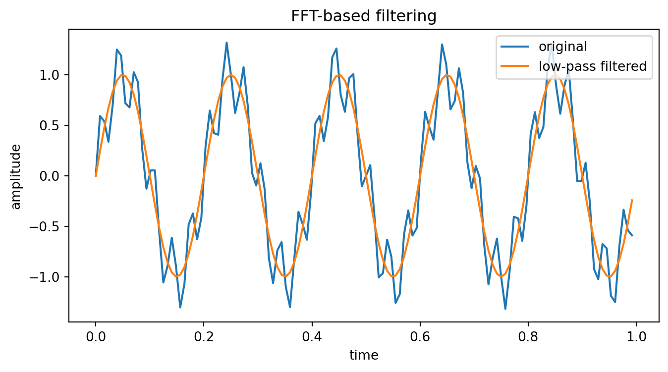
A common use of the FFT is filtering. The workflow is:
1. transform the signal into frequency coordinates;
2. modify some frequency coefficients;
3. transform back into time coordinates.
For example, a simple low-pass filter keeps low frequencies and removes high frequencies.
```{python}
import numpy as np
import matplotlib.pyplot as plt

n = 128
t = np.linspace(0, 1, n, endpoint=False)
signal = np.sin(2*np.pi*5*t) + 0.35*np.sin(2*np.pi*30*t)

F = np.fft.fft(signal)
filtered = F.copy()
# keep frequencies with index <= 8 and >= n-8, remove the rest
filtered[9:n-8] = 0
reconstructed = np.fft.ifft(filtered).real

plt.figure(figsize=(8, 4))
plt.plot(t, signal, label="original")
plt.plot(t, reconstructed, label="low-pass filtered")
plt.legend()
plt.xlabel("time")
plt.ylabel("amplitude")
plt.title("FFT-based filtering")
plt.show()
```
## 16. Circulant matrices and Fourier diagonalization
A circulant matrix is a matrix whose rows are cyclic shifts of one vector. For example,
$$
C=\begin{bmatrix}
c_0&c_{n-1}&c_{n-2}&\cdots&c_1\\
c_1&c_0&c_{n-1}&\cdots&c_2\\
\vdots&\vdots&\vdots&\ddots&\vdots\\
c_{n-1}&c_{n-2}&c_{n-3}&\cdots&c_0
\end{bmatrix}.
$$
::: {.callout-tip}
## Theorem 16.19: Circulant matrices are diagonalized by the Fourier basis
If $C\in\mathbb C^{n\times n}$ is circulant, then $C$ is diagonalized by the Fourier basis. Equivalently, there is a diagonal matrix $\Lambda$ such that
$$
C=F_n^{-1}\Lambda F_n.
$$
The diagonal entries of $\Lambda$ are obtained from the DFT of the first column of $C$.
:::
<details>
<summary><strong>Show proof idea</strong></summary>
A circulant matrix represents circular convolution. The Fourier basis vectors are eigenvectors of circular shifts because shifting a pure frequency only multiplies it by a complex phase. Since every circulant matrix is a linear combination of powers of the circular shift matrix, every Fourier basis vector is also an eigenvector of $C$. Thus $C$ is diagonal in the Fourier basis.
</details>
## 17. Practice problems
### Problem 1: Fourier matrix for $n=3$
Let $\omega_3=e^{-2\pi i/3}$. Write down the Fourier matrix $F_3$.
<details>
<summary><strong>Show solution</strong></summary>
The matrix is
$$
F_3=\begin{bmatrix}
1&1&1\\
1&\omega_3&\omega_3^2\\
1&\omega_3^2&\omega_3^4
\end{bmatrix}.
$$
Since $\omega_3^3=1$, $\omega_3^4=\omega_3$. Thus
$$
F_3=\begin{bmatrix}
1&1&1\\
1&\omega_3&\omega_3^2\\
1&\omega_3^2&\omega_3
\end{bmatrix}.
$$
</details>
### Problem 2: Constant signal
Let $\vec f=(2,2,2,2)^T$. Compute $F_4\vec f$.
<details>
<summary><strong>Show solution</strong></summary>
Since $\vec f=2(1,1,1,1)^T$ and $F_4(1,1,1,1)^T=(4,0,0,0)^T$,
$$
F_4\vec f=(8,0,0,0)^T.
$$
</details>
### Problem 3: Alternating signal
Let $\vec f=(3,-3,3,-3)^T$. Compute $F_4\vec f$.
<details>
<summary><strong>Show solution</strong></summary>
Since $\vec f=3(1,-1,1,-1)^T$ and $F_4(1,-1,1,-1)^T=(0,0,4,0)^T$,
$$
F_4\vec f=(0,0,12,0)^T.
$$
</details>
### Problem 4: Inverse DFT
If $\widehat{\vec f}=(4,0,0,0)^T$, find $\vec f$.
<details>
<summary><strong>Show solution</strong></summary>
Using $\vec f=\frac14F_4^*\widehat{\vec f}$, the result is
$$
\vec f=(1,1,1,1)^T.
$$
</details>
### Problem 5: Complexity comparison
Compare the order of direct DFT and FFT when $n=2^{20}$.
<details>
<summary><strong>Show solution</strong></summary>
Direct DFT costs about
$$
n^2=2^{40}
$$
operations. FFT costs about
$$
n\log_2 n=2^{20}\cdot 20.
$$
The ratio is approximately
$$
\frac{2^{40}}{20\cdot 2^{20}}=\frac{2^{20}}{20}\approx 52{,}428.
$$
</details>
## 18. Classical challenge questions
### Challenge 1: FFT is exact
Is the FFT an approximation to the DFT?
<details>
<summary><strong>Show answer</strong></summary>
No. The FFT computes exactly the same mathematical transformation as the DFT, except for ordinary floating-point roundoff. It is an algorithmic improvement, not a different transform.
</details>
### Challenge 2: Projection viewpoint
Explain why Fourier series is an orthogonal projection problem.
<details>
<summary><strong>Show answer</strong></summary>
A finite Fourier approximation chooses the best approximation to $f$ from the subspace spanned by finitely many orthogonal sine/cosine or complex exponential functions. The best approximation in $L^2$ is the orthogonal projection, and the Fourier coefficient formulas are exactly projection coefficients.
</details>
### Challenge 3: Why roots of unity matter
Why does the identity $1+q+\cdots+q^{n-1}=0$ appear in Fourier analysis?
<details>
<summary><strong>Show answer</strong></summary>
It proves orthogonality of distinct Fourier modes. Inner products between different columns of $F_n$ reduce to geometric sums of nontrivial roots of unity, which vanish.
</details>
### Challenge 4: Circulant matrices
Why does the Fourier basis diagonalize circulant matrices?
<details>
<summary><strong>Show answer</strong></summary>
Circulant matrices are combinations of cyclic shift matrices. Fourier vectors are eigenvectors of cyclic shifts, so they are simultaneously eigenvectors of all circulant matrices. Therefore circulant matrices become diagonal in the Fourier basis.
</details>
## 19. AI companion activities
Use an AI assistant as a study partner, not as a substitute for computation.
### Activity A: Explain in three languages
Ask:
> Explain the discrete Fourier transform in three ways: as a change of basis, as frequency measurement, and as multiplication by a matrix.
Then compare the answer with Definition 16.7 and Definition 16.8.
### Activity B: Debug a Fourier matrix
Ask the AI to write Python code to construct $F_n$. Then test whether the code satisfies
$$
F_n^*F_n=nI_n.
$$
If it does not, identify whether the issue is indexing, conjugation, or the sign convention.
### Activity C: FFT versus DFT
Ask:
> Why is FFT $O(n\log n)$ while direct DFT is $O(n^2)$?
Then write the recursion
$$
T(n)=2T(n/2)+O(n)
$$
by hand and solve it yourself.
### Activity D: Frequency filtering experiment
Use Python to create a signal with two frequencies. Ask the AI to suggest a low-pass filter, but verify the result by plotting the original and reconstructed signals.
## 20. Summary
- Fourier series expresses periodic functions in an orthogonal basis of waves.
- The Fourier transform extends the idea to nonperiodic functions.
- The DFT turns a finite data vector into frequency coordinates.
- The Fourier matrix satisfies $F_n^*F_n=nI_n$.
- The FFT computes the same DFT in $O(n\log n)$ operations.
- Fourier methods are central to signal processing, PDEs, convolution, image processing, and structured matrix computations.