---
title: "Chapter 20: Hilbert Spaces and Applications"
subtitle: "Infinite-Dimensional Linear Algebra for Signals, Probability, PDEs, and Machine Learning"
author: "He Wang"
format:
html:
toc: true
number-sections: true
code-fold: true
code-tools: true
jupyter: python3
---
# The story: when vectors become functions
In the first chapters of this course, a vector was often a column of numbers. Later, a vector became a polynomial, a matrix, a signal, or a state of a system. Chapter 20 makes this viewpoint explicit:
> A vector can be any object that supports addition, scalar multiplication, length, angle, projection, and approximation.
The main challenge is that many natural spaces are infinite-dimensional. For example, a signal is a function, and a function may require infinitely many coordinates. To do linear algebra safely in such spaces, we need one extra idea:
> **Completeness:** Cauchy sequences should have limits inside the space.
A **Hilbert space** is an inner product space that is complete. This one definition is the bridge from finite-dimensional linear algebra to Fourier analysis, least squares, probability, differential equations, quantum mechanics, and kernel methods.
## Learning goals
By the end of this chapter, you should be able to:
1. distinguish metric, normed, Banach, inner product, and Hilbert spaces;
2. explain why completeness matters;
3. compute projections using Gram matrices;
4. interpret Fourier coefficients as coordinates in a Hilbert space;
5. understand why $L^2$ identifies functions that differ only on sets of measure zero;
6. state and use the Riesz representation theorem;
7. connect kernels and RKHS ideas to linear algebra.
# From finite-dimensional geometry to Hilbert spaces
In $\mathbb{R}^n$, the dot product gives length, angle, orthogonality, projection, and least squares. The guiding question is:
> Which infinite-dimensional spaces still allow the same geometry?
The answer is: **Hilbert spaces**.
::: {.callout-tip}
## Big idea
Finite-dimensional linear algebra teaches us geometry. Hilbert space theory keeps the same geometry but allows infinite coordinates and limiting processes.
:::
# A hierarchy of spaces
The following hierarchy is useful:
$$
\text{set}
\supset
\text{metric space}
\supset
\text{normed vector space}
\supset
\text{inner product space}
\supset
\text{Hilbert space}.
$$
There is also another branch:
$$
\text{complete normed vector space}=\text{Banach space}.
$$
A Hilbert space is both an inner product space and a Banach space, with the norm coming from the inner product.
## Definition: metric space
A **metric space** is a set $S$ with a distance function
$$
d:S\times S\to \mathbb{R}
$$
such that for all $x,y,z\in S$,
1. $d(x,y)\ge 0$ and $d(x,y)=0$ if and only if $x=y$;
2. $d(x,y)=d(y,x)$;
3. $d(x,z)\le d(x,y)+d(y,z)$.
## Definition: Cauchy sequence and completeness
A sequence $(x_n)$ in a metric space is **Cauchy** if for every $\varepsilon>0$, there exists $N$ such that
$$
d(x_m,x_n)<\varepsilon
\qquad\text{whenever }m,n\ge N.
$$
A metric space is **complete** if every Cauchy sequence converges to a point in the space.
::: {.callout-note collapse="true"}
## Proof/intuition: why Cauchy sequences matter
A Cauchy sequence is a sequence whose terms eventually become arbitrarily close to each other. It is trying to converge. Completeness says that whenever a sequence is internally convergent in this sense, the limit is not missing from the space.
For example, $\mathbb{Q}$ is not complete because rational approximations can converge to $\sqrt{2}$, which is not rational.
:::
## Definition: normed vector space and Banach space
A **norm** on a vector space $V$ is a function
$$
\|\cdot\|:V\to\mathbb{R}
$$
such that for all $u,v\in V$ and scalars $c$,
1. $\|v\|\ge 0$ and $\|v\|=0$ if and only if $v=0$;
2. $\|cv\|=|c|\|v\|$;
3. $\|u+v\|\le \|u\|+\|v\|$.
A complete normed vector space is called a **Banach space**.
## Definition: inner product space
A real inner product on a vector space $V$ is a function
$$
\langle\cdot,\cdot\rangle:V\times V\to \mathbb{R}
$$
such that for all $u,v,w\in V$ and $c\in\mathbb{R}$,
1. $\langle u,v\rangle=\langle v,u\rangle$;
2. $\langle u+v,w\rangle=\langle u,w\rangle+\langle v,w\rangle$;
3. $\langle cu,v\rangle=c\langle u,v\rangle$;
4. $\langle v,v\rangle\ge 0$, and $\langle v,v\rangle=0$ if and only if $v=0$.
For complex spaces, symmetry is replaced by conjugate symmetry:
$$
\langle u,v\rangle=\overline{\langle v,u\rangle}.
$$
The norm induced by an inner product is
$$
\|v\|=\sqrt{\langle v,v\rangle}.
$$
## Example: matrix inner product
The space $\mathbb{R}^{m\times n}$ has the Frobenius inner product
$$
\langle A,B\rangle=\operatorname{tr}(AB^T)=\sum_{i=1}^m\sum_{j=1}^n a_{ij}b_{ij}.
$$
The induced norm is
$$
\|A\|_F=\sqrt{\sum_{i,j}a_{ij}^2}.
$$
## Example: random variables as vectors
Let $X$ and $Y$ be real random variables with finite second moments. Then
$$
\langle X,Y\rangle=\mathbb{E}(XY)
$$
is an inner product after identifying random variables that are equal almost surely. The induced norm is
$$
\|X\|_2=\sqrt{\mathbb{E}(X^2)}.
$$
This is one reason least squares and regression are naturally Hilbert space ideas.
# Hilbert spaces
## Definition: Hilbert space
A **Hilbert space** is a complete inner product space.
A Hilbert space is a space where all the finite-dimensional geometric tools still work and where infinite limits are allowed.
## Example: finite-dimensional Hilbert spaces
Every finite-dimensional inner product space over $\mathbb{R}$ or $\mathbb{C}$ is complete. Therefore $\mathbb{R}^n$ and $\mathbb{C}^n$ are Hilbert spaces with their standard inner products.
## Example: the sequence space $\ell^2$
The space
$$
\ell^2=\left\{x=(x_1,x_2,\ldots):\sum_{n=1}^{\infty}|x_n|^2<\infty\right\}
$$
with inner product
$$
\langle x,y\rangle=\sum_{n=1}^{\infty}x_n\overline{y_n}
$$
is a Hilbert space.
Its standard orthonormal basis is
$$
e_1=(1,0,0,\ldots),\quad e_2=(0,1,0,\ldots),\quad \ldots
$$
Every $x\in \ell^2$ has the expansion
$$
x=\sum_{n=1}^{\infty}x_ne_n,
$$
where convergence is in the $\ell^2$ norm.
## Example: $L^2[-\pi,\pi]$
The function space
$$
L^2[-\pi,\pi]
=
\left\{
f:\int_{-\pi}^{\pi}|f(x)|^2\,dx<\infty
\right\}
$$
has inner product
$$
\langle f,g\rangle
=
\int_{-\pi}^{\pi}f(x)\overline{g(x)}\,dx.
$$
After identifying functions that agree except on a set of measure zero, $L^2[-\pi,\pi]$ is a Hilbert space.
::: {.callout-warning}
## Important subtlety
In $L^2$, a vector is not exactly one function formula. It is an equivalence class of functions that agree almost everywhere.
:::
# A non-example: polynomials are not complete
Let
$$
\mathcal{P}
=
\{\text{all real polynomials on }[0,1]\}
$$
with inner product
$$
\langle f,g\rangle=\int_0^1 f(t)g(t)\,dt.
$$
This is an inner product space, but it is not a Hilbert space.
## Proposition
The space $\mathcal{P}$ of all polynomials on $[0,1]$ with the $L^2$ inner product is not complete.
::: {.callout-note collapse="true"}
## Proof
Consider the partial Taylor polynomials
$$
p_m(x)=\sum_{k=0}^{m}\frac{x^k}{k!}.
$$
For $n>m$,
$$
p_n-p_m=\sum_{k=m+1}^{n}\frac{x^k}{k!}.
$$
Using the triangle inequality in the $L^2$ norm,
$$
\|p_n-p_m\|_{L^2}
\le
\sum_{k=m+1}^{n}
\left\|\frac{x^k}{k!}\right\|_{L^2}.
$$
But
$$
\left\|\frac{x^k}{k!}\right\|_{L^2}
=
\frac{1}{k!}
\left(\int_0^1 x^{2k}\,dx\right)^{1/2}
=
\frac{1}{k!\sqrt{2k+1}}.
$$
The series
$$
\sum_{k=0}^{\infty}\frac{1}{k!\sqrt{2k+1}}
$$
converges. Hence $(p_m)$ is Cauchy in the $L^2$ norm.
However, $p_m\to e^x$ uniformly on $[0,1]$, hence also in $L^2[0,1]$. The function $e^x$ is not a polynomial. Therefore the Cauchy sequence $(p_m)$ does not converge to an element of $\mathcal{P}$. Thus $\mathcal{P}$ is not complete.
:::
## Remark
For a fixed degree $d$, the space
$$
\mathcal{P}_d=\{\text{polynomials of degree at most }d\}
$$
is finite-dimensional. Hence it is complete and is a Hilbert space with the $L^2$ inner product.
# Orthogonal projection and least squares
The most important reason Hilbert spaces are useful is the projection theorem. It is the infinite-dimensional version of least squares.
## Theorem: orthogonal projection theorem
Let $\mathcal{H}$ be a Hilbert space and let $\mathcal{M}\subseteq \mathcal{H}$ be a closed linear subspace. For every $y\in\mathcal{H}$, there exists a unique element $p\in\mathcal{M}$ such that
$$
\|y-p\|=\min_{w\in\mathcal{M}}\|y-w\|.
$$
Moreover, $p$ is characterized by the orthogonality condition
$$
y-p\perp \mathcal{M},
$$
meaning
$$
\langle y-p,w\rangle=0
\qquad
\text{for all }w\in\mathcal{M}.
$$
We write
$$
p=\operatorname{Proj}_{\mathcal{M}}y.
$$
::: {.callout-note collapse="true"}
## Proof idea
The finite-dimensional proof says: find the closest point, then show the residual is orthogonal to the subspace.
In an infinite-dimensional Hilbert space, the difficulty is existence of a closest point. Choose a minimizing sequence $(w_n)$ in $\mathcal{M}$ such that
$$
\|y-w_n\|\to \inf_{w\in \mathcal{M}}\|y-w\|.
$$
Using the parallelogram identity, one proves that $(w_n)$ is Cauchy. Since $\mathcal{H}$ is complete and $\mathcal{M}$ is closed, $w_n$ converges to some $p\in\mathcal{M}$. This $p$ is the minimizer.
The orthogonality condition follows by minimizing
$$
\phi(t)=\|y-(p+tw)\|^2
$$
for arbitrary $w\in\mathcal{M}$. Since $p$ is closest, $t=0$ is a minimum, so $\phi'(0)=0$, which gives $\langle y-p,w\rangle=0$.
:::
## Projection onto a finite-dimensional subspace
Let
$$
\mathcal{M}=\operatorname{span}\{u_1,\ldots,u_m\}
$$
inside a Hilbert space $\mathcal{H}$. If
$$
p=c_1u_1+\cdots+c_mu_m,
$$
then the condition $y-p\perp \mathcal{M}$ gives
$$
\langle y-p,u_i\rangle=0,
\qquad i=1,\ldots,m.
$$
Therefore
$$
\sum_{j=1}^{m}c_j\langle u_j,u_i\rangle=\langle y,u_i\rangle.
$$
In matrix form,
$$
G\mathbf{c}=\mathbf{b},
$$
where
$$
G_{ij}=\langle u_j,u_i\rangle,
\qquad
b_i=\langle y,u_i\rangle.
$$
This is the Hilbert-space normal equation.
# Orthonormal systems and Fourier viewpoint
## Definition: orthonormal set
A collection $\{e_i\}_{i\in I}$ in an inner product space is **orthonormal** if
$$
\langle e_i,e_j\rangle
=
\begin{cases}
1,&i=j,\\
0,&i\ne j.
\end{cases}
$$
## Proposition
Every orthonormal set is linearly independent.
::: {.callout-note collapse="true"}
## Proof
Suppose
$$
c_1e_1+\cdots+c_me_m=0.
$$
Taking the inner product with $e_j$ gives
$$
c_j=
\langle c_1e_1+\cdots+c_me_m,e_j\rangle
=
\langle 0,e_j\rangle
=
0.
$$
Thus all coefficients are zero.
:::
## Theorem: Bessel inequality
Let $\{e_1,e_2,\ldots\}$ be an orthonormal sequence in a Hilbert space $\mathcal{H}$. Then for every $f\in\mathcal{H}$,
$$
\sum_{n=1}^{\infty}|\langle f,e_n\rangle|^2
\le
\|f\|^2.
$$
::: {.callout-note collapse="true"}
## Proof
For each $N$, let
$$
p_N=\sum_{n=1}^{N}\langle f,e_n\rangle e_n.
$$
Then $p_N$ is the orthogonal projection of $f$ onto $\operatorname{span}\{e_1,\ldots,e_N\}$. Therefore
$$
\|f\|^2=\|p_N\|^2+\|f-p_N\|^2\ge \|p_N\|^2.
$$
Since the $e_n$ are orthonormal,
$$
\|p_N\|^2=\sum_{n=1}^{N}|\langle f,e_n\rangle|^2.
$$
Letting $N\to\infty$ gives the result.
:::
## Definition: Hilbert basis
An orthonormal sequence $\{e_n\}$ is a **Hilbert basis**, or **complete orthonormal basis**, if every $f\in\mathcal{H}$ can be written as
$$
f=\sum_{n=1}^{\infty}\langle f,e_n\rangle e_n
$$
with convergence in the Hilbert space norm.
## Theorem: Parseval identity
If $\{e_n\}$ is a Hilbert basis for $\mathcal{H}$, then
$$
\|f\|^2=\sum_{n=1}^{\infty}|\langle f,e_n\rangle|^2.
$$
## Example: Fourier basis
In $L^2[-\pi,\pi]$, the functions
$$
e_k(x)=\frac{1}{\sqrt{2\pi}}e^{ikx},
\qquad k\in\mathbb{Z},
$$
form an orthonormal basis. The Fourier coefficient of $f$ is
$$
\widehat f(k)=
\langle f,e_k\rangle
=
\frac{1}{\sqrt{2\pi}}
\int_{-\pi}^{\pi}f(x)e^{-ikx}\,dx.
$$
Thus Fourier series are coordinate expansions in a Hilbert space.
# Riesz representation theorem
The dual space of a finite-dimensional inner product space is naturally identified with the original space. The same remains true in Hilbert spaces if we restrict to continuous linear functionals.
## Definition: bounded linear functional
Let $\mathcal{H}$ be a Hilbert space. A linear functional
$$
L:\mathcal{H}\to \mathbb{R}
\quad\text{or}\quad
L:\mathcal{H}\to \mathbb{C}
$$
is **bounded** if there exists $C>0$ such that
$$
|L(f)|\le C\|f\|
$$
for all $f\in\mathcal{H}$.
## Theorem: Riesz representation theorem
Let $\mathcal{H}$ be a Hilbert space. For every bounded linear functional $L$ on $\mathcal{H}$, there exists a unique vector $g\in\mathcal{H}$ such that
$$
L(f)=\langle f,g\rangle
$$
for all $f\in\mathcal{H}$.
::: {.callout-note collapse="true"}
## Proof idea
If $L=0$, take $g=0$. Otherwise, $\ker L$ is a closed subspace of $\mathcal{H}$. Choose a unit vector
$$
u\in(\ker L)^\perp.
$$
Every $f\in\mathcal{H}$ decomposes as
$$
f=w+\alpha u,
\qquad w\in\ker L.
$$
Then $L(f)=\alpha L(u)$, and $\alpha=\langle f,u\rangle$. Therefore
$$
L(f)=\langle f,\overline{L(u)}u\rangle
$$
under the convention that the inner product is linear in the first variable. Uniqueness follows by testing the difference of two representing vectors against itself.
:::
## Example: integral functionals
Let $\mathcal{H}=L^2[0,1]$ and fix $g\in L^2[0,1]$. Then
$$
L(f)=\int_0^1 f(x)g(x)\,dx
$$
is a bounded linear functional. Riesz says that every bounded linear functional on $L^2[0,1]$ has this form for a unique $g\in L^2[0,1]$.
# Why $L^2$ uses equivalence classes
The natural function Hilbert spaces are built using the Lebesgue integral. The reason is that Cauchy sequences of nice functions often converge to less nice functions.
## Definition: positive and negative parts
For a real-valued function $f$, define
$$
f_+(x)=\max\{f(x),0\},
\qquad
f_-(x)=\max\{-f(x),0\}.
$$
Then
$$
f=f_+-f_-,
\qquad
|f|=f_++f_-.
$$
## Definition: $L^2$ equivalence
Two measurable functions $f,g$ are identified in $L^2$ if
$$
\int |f-g|^2=0.
$$
Equivalently, they are equal except on a set of measure zero.
## Example: changing one value
Let $f(x)=0$ on $[0,1]$. Define $g$ by
$$
g(1/2)=100,
\qquad
g(x)=0 \text{ otherwise}.
$$
Then
$$
\int_0^1 |f(x)-g(x)|^2\,dx=0.
$$
Thus $f$ and $g$ represent the same vector in $L^2[0,1]$.
# Kernel viewpoint and RKHS
A kernel is a function that behaves like an inner product after mapping data into a Hilbert space. This idea connects Hilbert spaces with modern machine learning.
## Definition: positive semidefinite kernel
Let $X$ be a set. A function
$$
K:X\times X\to\mathbb{R}
$$
is a **positive semidefinite kernel** if for any $x_1,\ldots,x_m\in X$, the Gram matrix
$$
G=[K(x_i,x_j)]_{i,j=1}^{m}
$$
is positive semidefinite.
## Example: polynomial kernel
For $x,y\in\mathbb{R}^d$, the function
$$
K(x,y)=(1+x^Ty)^r
$$
is a positive semidefinite kernel. It corresponds to taking inner products after mapping $x$ into a larger feature space of monomials up to degree $r$.
## Definition: reproducing kernel Hilbert space
A Hilbert space $\mathcal{H}$ of functions on a set $X$ is called a **reproducing kernel Hilbert space** if for every $x\in X$, evaluation at $x$ is a bounded linear functional. By the Riesz theorem, there exists $K_x\in\mathcal{H}$ such that
$$
f(x)=\langle f,K_x\rangle
\qquad
\text{for all }f\in\mathcal{H}.
$$
The function
$$
K(x,y)=K_y(x)
$$
is called the **reproducing kernel**.
::: {.callout-tip}
## Linear algebra interpretation
The equation
$$
f(x)=\langle f,K_x\rangle
$$
says that evaluating a function is the same as taking an inner product with a special vector $K_x$.
:::
# Applications
## Fourier analysis
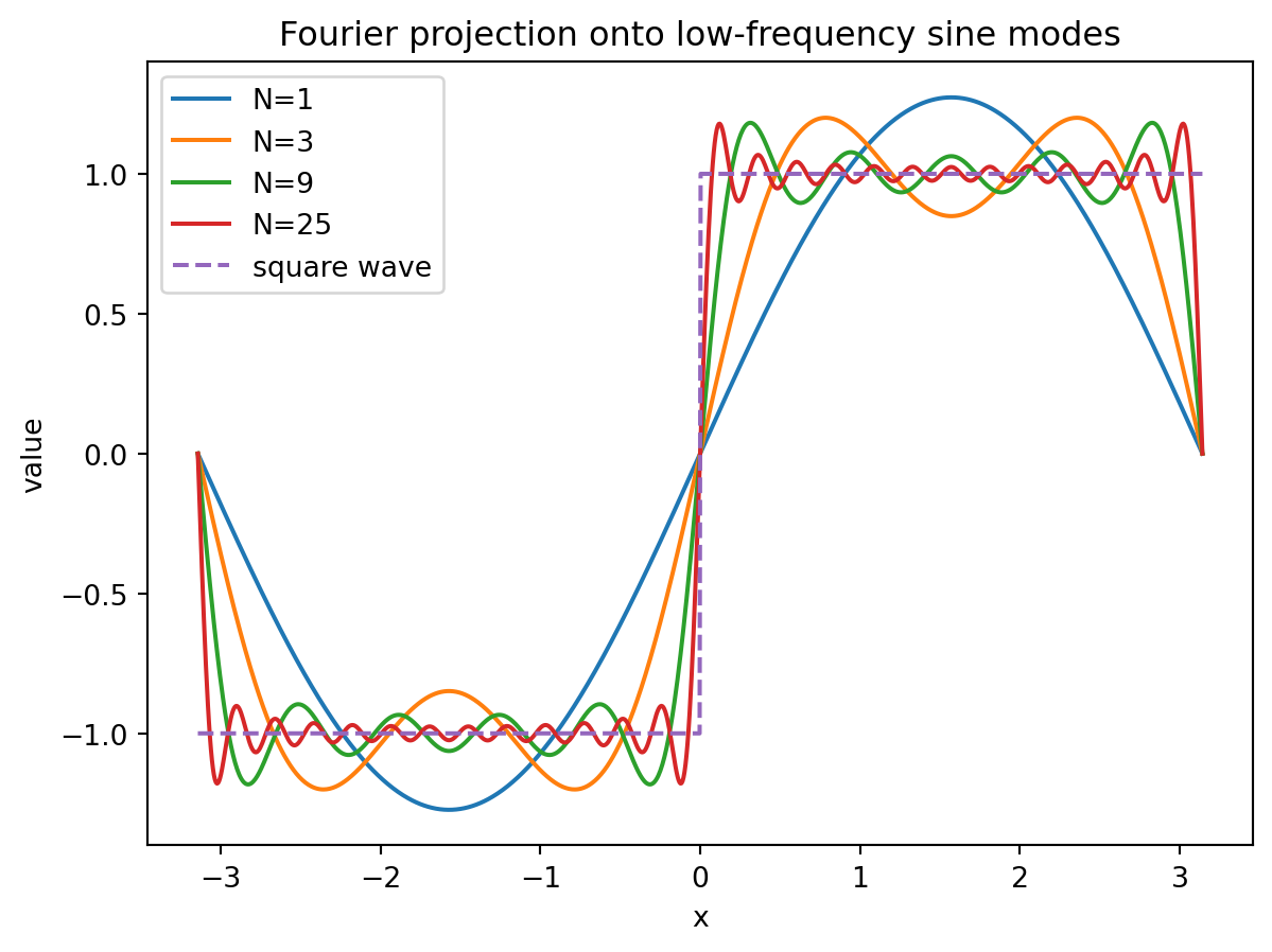
In $L^2[-\pi,\pi]$, the Fourier basis decomposes a signal into orthogonal frequency directions. Projection onto a finite-dimensional subspace
$$
\operatorname{span}\{e^{-iNx},\ldots,e^{iNx}\}
$$
gives a low-frequency approximation of the signal.
## Probability and statistics
Random variables with finite variance form a Hilbert space. Orthogonal projection becomes conditional expectation:
$$
\mathbb{E}(Y\mid X)
$$
is the projection of $Y$ onto the closed subspace of functions of $X$. This is the Hilbert space foundation of least squares regression.
## PDEs and weak solutions
Many differential equations are solved not by searching for classical derivatives, but by searching in a Hilbert space such as $L^2$ or a Sobolev space. The equation is tested against all vectors in a space, producing a weak formulation.
## Quantum mechanics
A quantum state is modeled by a unit vector in a complex Hilbert space. Observables are represented by self-adjoint linear operators. Orthogonal projection describes measurement onto a subspace of possible states.
## Kernel methods
Support vector machines, Gaussian processes, and kernel ridge regression use kernels to perform linear algebra in high-dimensional or infinite-dimensional Hilbert spaces without explicitly writing the feature map.
# Python computation 1: projection in a finite-dimensional Hilbert space
This computation projects a vector onto the span of two non-orthonormal vectors.
```{python}
import numpy as np

v1 = np.array([1.0, 1.0, 0.0])
v2 = np.array([1.0, 0.0, 1.0])
y  = np.array([2.0, 1.0, 3.0])

A = np.column_stack([v1, v2])

# Projection onto im(A): A(A^T A)^{-1}A^T y
proj = A @ np.linalg.solve(A.T @ A, A.T @ y)
residual = y - proj

print("Projection:", proj)
print("Residual:", residual)
print("A^T residual:", A.T @ residual)
```
The last line should be approximately zero. This verifies the orthogonality condition.
# Python computation 2: best quadratic approximation to $e^x$
We approximate $e^x$ on $[0,1]$ by a quadratic polynomial
$$
p(x)=c_0+c_1x+c_2x^2
$$
using the $L^2$ inner product.
The normal equations are
$$
G\mathbf{c}=\mathbf{b},
$$
where
$$
G_{ij}=\int_0^1 x^{i+j}\,dx,
\qquad
b_i=\int_0^1 e^x x^i\,dx.
$$
```{python}
import sympy as sp

x = sp.symbols("x")
basis = [1, x, x**2]
f = sp.exp(x)

G = sp.Matrix([[sp.integrate(basis[j]*basis[i], (x, 0, 1))
                for j in range(3)] for i in range(3)])

rhs = sp.Matrix([sp.integrate(f*basis[i], (x, 0, 1)) for i in range(3)])

c = G.LUsolve(rhs)
p = sp.expand(sum(c[i]*basis[i] for i in range(3)))

G, rhs, [sp.simplify(ci) for ci in c], p
```
```{python}
# Numerical values
[float(ci) for ci in c]
```
# Python computation 3: Fourier coefficients as coordinates
We approximate a square wave using finitely many sine terms.
```{python}
import numpy as np
import matplotlib.pyplot as plt

xs = np.linspace(-np.pi, np.pi, 1000)
f = np.sign(np.sin(xs))

def fourier_square(xs, N):
    s = np.zeros_like(xs)
    for k in range(1, N+1, 2):
        s += (4/np.pi) * np.sin(k*xs)/k
    return s

for N in [1, 3, 9, 25]:
    plt.plot(xs, fourier_square(xs, N), label=f"N={N}")

plt.plot(xs, f, "--", label="square wave")
plt.legend()
plt.title("Fourier projection onto low-frequency sine modes")
plt.xlabel("x")
plt.ylabel("value")
plt.show()
```
# Challenge questions
## Challenge 1: why closed subspaces matter
Explain why the projection theorem can fail if the subspace is not closed. Use the polynomial subspace of $L^2[0,1]$ as an intuitive example.
::: {.callout-note collapse="true"}
## Solution
Let $\mathcal{H}=L^2[0,1]$ and let $\mathcal{M}$ be the space of polynomials. The polynomial space is dense in $L^2[0,1]$, but it is not closed.
Take a function $f\in L^2[0,1]$ that is not a polynomial, such as $f(x)=e^x$. Since polynomials are dense,
$$
\inf_{p\in\mathcal{M}}\|f-p\|_{L^2}=0.
$$
But no polynomial equals $f$ as an $L^2$ vector. Therefore there is no closest polynomial in $\mathcal{M}$. The infimum is zero but is not attained.
:::
## Challenge 2: projection from Gram matrices
Let $\mathcal{M}=\operatorname{span}\{u_1,\ldots,u_m\}$ in a Hilbert space. Derive the system for the coefficients of $\operatorname{Proj}_{\mathcal{M}}y$.
::: {.callout-note collapse="true"}
## Solution
Write
$$
p=c_1u_1+\cdots+c_mu_m.
$$
The projection condition is
$$
y-p\perp \mathcal{M}.
$$
It is enough to impose
$$
\langle y-p,u_i\rangle=0,\qquad i=1,\ldots,m.
$$
Thus
$$
\langle y,u_i\rangle
=
\sum_{j=1}^{m}c_j\langle u_j,u_i\rangle.
$$
This is the Gram system
$$
G\mathbf{c}=\mathbf{b}.
$$
:::
## Challenge 3: Fourier coefficients as coordinates
Let $\{e_n\}$ be an orthonormal basis for a Hilbert space. Explain why $\langle f,e_n\rangle$ is the $n$-th coordinate of $f$.
::: {.callout-note collapse="true"}
## Solution
If
$$
f=\sum_{n=1}^{\infty}c_ne_n,
$$
then taking the inner product with $e_j$ gives
$$
\langle f,e_j\rangle
=
\sum_{n=1}^{\infty}c_n\langle e_n,e_j\rangle
=
c_j.
$$
Thus $\langle f,e_j\rangle$ is exactly the $j$-th coordinate of $f$.
:::
# Practice problems
## Problem 1
Let $u_1=(1,1,0)$, $u_2=(1,0,1)$, and $y=(2,1,3)$ in $\mathbb{R}^3$. Find the projection of $y$ onto $\operatorname{span}\{u_1,u_2\}$.
::: {.callout-note collapse="true"}
## Solution
Let $A=[u_1\ u_2]$. Then
$$
p=A(A^TA)^{-1}A^Ty.
$$
Here
$$
A=
\begin{bmatrix}
1&1\\
1&0\\
0&1
\end{bmatrix}.
$$
Compute
$$
A^TA=
\begin{bmatrix}
2&1\\
1&2
\end{bmatrix},
\qquad
A^Ty=
\begin{bmatrix}
3\\
5
\end{bmatrix}.
$$
Solving gives
$$
\begin{bmatrix}
2&1\\
1&2
\end{bmatrix}
\begin{bmatrix}
c_1\\c_2
\end{bmatrix}
=
\begin{bmatrix}
3\\5
\end{bmatrix}.
$$
Thus $c_1=\frac13$ and $c_2=\frac73$. Therefore
$$
p=\frac13u_1+\frac73u_2
=
\left(\frac83,\frac13,\frac73\right).
$$
:::
## Problem 2
Show that the sequence $x=(1,\frac12,\frac13,\ldots)$ is not in $\ell^2$, but $y=(1,\frac12,\frac14,\frac18,\ldots)$ is in $\ell^2$.
::: {.callout-note collapse="true"}
## Solution
For $x$,
$$
\sum_{n=1}^{\infty}\left|\frac1n\right|^2
=
\sum_{n=1}^{\infty}\frac1{n^2}
<\infty.
$$
So $x$ actually is in $\ell^2$.
For $y$,
$$
\sum_{n=0}^{\infty}\left(\frac1{2^n}\right)^2
=
\sum_{n=0}^{\infty}\frac1{4^n}
=
\frac{1}{1-\frac14}
=
\frac43.
$$
So $y\in \ell^2$.
A correct nonexample is $z=(1,\frac1{\sqrt2},\frac1{\sqrt3},\ldots)$, since
$$
\sum_{n=1}^{\infty}\frac1n
$$
diverges.
:::
## Problem 3
Let $L(f)=\int_0^1 f(x)x^2\,dx$ on $L^2[0,1]$. Find the Riesz representing vector.
::: {.callout-note collapse="true"}
## Solution
The Riesz representation theorem says that
$$
L(f)=\langle f,g\rangle
$$
for a unique $g\in L^2[0,1]$. Since
$$
L(f)=\int_0^1 f(x)x^2\,dx,
$$
we have
$$
g(x)=x^2.
$$
:::
# AI companion activities
Use AI as a study partner, not as a replacement for your own reasoning.
## Activity 1: explain the hierarchy
Ask an AI tool:
> Explain the difference between metric spaces, normed spaces, Banach spaces, inner product spaces, and Hilbert spaces using examples from linear algebra.
Then check whether the answer correctly says that every Hilbert space is a Banach space, but not every Banach space is a Hilbert space.
## Activity 2: generate projection examples
Ask:
> Give me three examples of orthogonal projection: one in $\mathbb{R}^3$, one in a polynomial space, and one in $L^2[0,1]$.
Verify each example by checking the residual is orthogonal to the subspace.
## Activity 3: connect Fourier series and coordinates
Ask:
> Explain Fourier coefficients as coordinates in an infinite-dimensional Hilbert space.
Then write your own one-paragraph explanation.
## Activity 4: kernel methods
Ask:
> Explain how a positive semidefinite kernel acts like an inner product in a hidden feature space.
Then test the idea numerically by constructing a Gram matrix from a kernel and checking its eigenvalues.
# Summary
Hilbert spaces are infinite-dimensional linear algebra spaces with enough completeness to support limits, projections, and approximations.
The main ideas are:
- A Hilbert space is a complete inner product space.
- Orthogonal projection generalizes least squares.
- Orthonormal bases generalize coordinate systems.
- Fourier series are Hilbert space coordinate expansions.
- Riesz representation identifies continuous linear functionals with inner products.
- $L^2$ spaces are central examples in analysis, probability, PDEs, signal processing, and machine learning.