# Lab 16: Fast Fourier Transforms {.unnumbered}
This independent-study lab accompanies Chapter 16. It focuses on the discrete Fourier transform, Fourier matrices, frequency interpretation, FFT recursion, and simple filtering.
## Learning goals
By the end of this lab, you should be able to:
1. construct the Fourier matrix $F_n$;
2. compute a DFT by matrix multiplication and by `np.fft.fft`;
3. verify $F_n^*F_n=nI_n$;
4. interpret impulse, constant, and alternating signals in the frequency domain;
5. explain the even-odd recursion behind the FFT;
6. apply a simple frequency-domain filter.
## Python practice notebook
Use the Jupyter notebook version for longer Python practice:
- [Download Lab 16 notebook](lab-16-fast-fourier-transforms-independent-study.ipynb)
- [Open Lab 16 in Google Colab](https://colab.research.google.com/github/wanghemath/MATH5110/blob/main/Labs/lab-16-fast-fourier-transforms-independent-study.ipynb)
If your book is hosted on GitHub, you can also add a Colab link:
[Open in Google Colab](https://colab.research.google.com/github/wanghemath/MATH5110/blob/main/labs/lab-16-fast-fourier-transforms-independent-study.ipynb)
## Interactive lab
Open the interactive HTML page:
[Open Lab 16 interactive page](lab-16-interactive.html)
The interactive page lets you edit a length-8 signal, compute its DFT, compare direct DFT with FFT-style recursion, and explore low-pass filtering.
## Key formulas
Let
$$
\omega_n=e^{-2\pi i/n}.
$$
The DFT of $\vec f=(f_0,\ldots,f_{n-1})^T$ is
$$
\widehat f_k=\sum_{j=0}^{n-1}f_j\omega_n^{jk}.
$$
The Fourier matrix is
$$
F_n=[\omega_n^{jk}]_{j,k=0}^{n-1},
\qquad
\widehat{\vec f}=F_n\vec f.
$$
The inverse DFT is
$$
\vec f=\frac1nF_n^*\widehat{\vec f}.
$$
For $n=2m$, the FFT recursion is
$$
\widehat f_k=\widehat f^{\,e}_k+\omega_n^k\widehat f^{\,o}_k,
\qquad
\widehat f_{k+m}=\widehat f^{\,e}_k-\omega_n^k\widehat f^{\,o}_k.
$$
## Part 1: Construct the Fourier matrix
```{python}
import numpy as np

def fourier_matrix(n):
    omega = np.exp(-2j*np.pi/n)
    return np.array([[omega**(j*k) for k in range(n)] for j in range(n)])

F4 = fourier_matrix(4)
print(np.round(F4, 3))
```
### Check your understanding
What is $\omega_4$? Why do powers of $\omega_4$ produce the entries $1,-i,-1,i$?
<details>
<summary><strong>Show answer</strong></summary>
Since
$$
\omega_4=e^{-2\pi i/4}=e^{-\pi i/2}=-i,
$$
its powers are
$$
1,\ -i,\ (-i)^2=-1,\ (-i)^3=i,
$$
and then the pattern repeats.
</details>
## Part 2: Verify orthogonality
```{python}
n = 8
F = fourier_matrix(n)
print(np.round(F.conj().T @ F, 8))
print(np.allclose(F.conj().T @ F, n*np.eye(n)))
```
### Practice question
Explain why $F_n^{-1}=\frac1nF_n^*$.
<details>
<summary><strong>Show answer</strong></summary>
The columns of $F_n$ are orthogonal and each has squared norm $n$. Therefore
$$
F_n^*F_n=nI_n.
$$
Multiplying by $1/n$ gives
$$
\left(\frac1nF_n^*\right)F_n=I_n.
$$
Since $F_n$ is square, $\frac1nF_n^*$ is the inverse.
</details>
## Part 3: DFT by matrix multiplication
```{python}
f = np.array([1, 2, 0, -1, 0, 1, 0, 0], dtype=complex)
F = fourier_matrix(len(f))
fhat_matrix = F @ f
fhat_numpy = np.fft.fft(f)

print("Matrix DFT:", np.round(fhat_matrix, 4))
print("NumPy FFT:  ", np.round(fhat_numpy, 4))
print("Same?", np.allclose(fhat_matrix, fhat_numpy))
```
## Part 4: Interpret three basic signals
```{python}
signals = {
    "impulse": np.array([1,0,0,0], dtype=complex),
    "constant": np.array([1,1,1,1], dtype=complex),
    "alternating": np.array([1,-1,1,-1], dtype=complex),
}

F4 = fourier_matrix(4)
for name, x in signals.items():
    print(name, "->", np.round(F4 @ x, 4))
```
### Similar practice question
Compute the DFT of $(2,2,2,2)^T$ and $(3,-3,3,-3)^T$.
<details>
<summary><strong>Show answer</strong></summary>
By scaling,
$$
F_4(2,2,2,2)^T=(8,0,0,0)^T,
$$
and
$$
F_4(3,-3,3,-3)^T=(0,0,12,0)^T.
$$
</details>
## Part 5: A recursive FFT
```{python}
def fft_recursive(f):
    f = np.asarray(f, dtype=complex)
    n = len(f)
    if n == 1:
        return f
    if n % 2 != 0:
        raise ValueError("This simple recursive FFT requires length a power of 2.")
    even = fft_recursive(f[::2])
    odd = fft_recursive(f[1::2])
    twiddle = np.exp(-2j*np.pi*np.arange(n//2)/n)
    top = even + twiddle * odd
    bottom = even - twiddle * odd
    return np.concatenate([top, bottom])

x = np.array([1, 2, 0, -1, 0, 1, 0, 0], dtype=complex)
print(np.round(fft_recursive(x), 4))
print(np.allclose(fft_recursive(x), np.fft.fft(x)))
```
### Reflection question
Why does the recursive FFT have complexity $O(n\log n)$?
<details>
<summary><strong>Show answer</strong></summary>
At each level, the algorithm splits the problem into two problems of size $n/2$, plus $O(n)$ work to combine the even and odd transforms. Therefore
$$
T(n)=2T(n/2)+O(n).
$$
There are $\log_2 n$ levels and each level costs $O(n)$ total work, so the total cost is $O(n\log n)$.
</details>
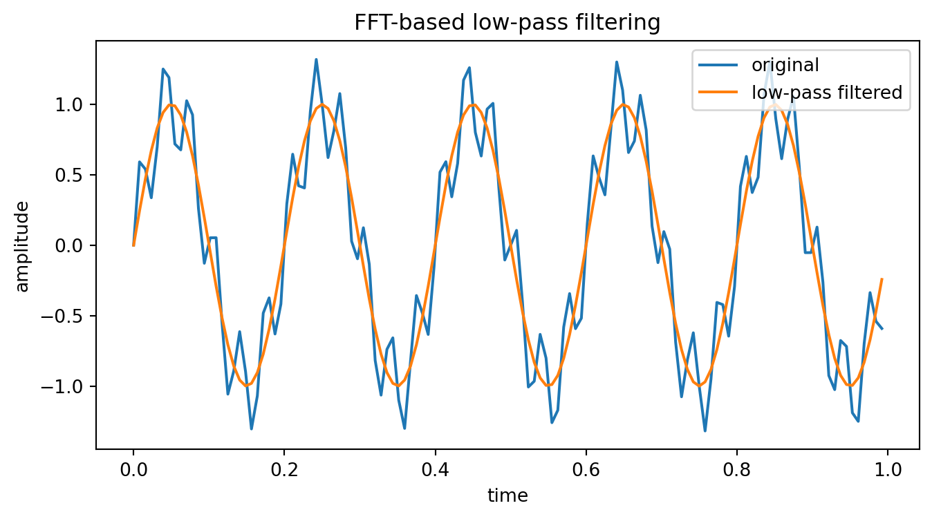
## Part 6: Frequency filtering
```{python}
import matplotlib.pyplot as plt

n = 128
t = np.linspace(0, 1, n, endpoint=False)
signal = np.sin(2*np.pi*5*t) + 0.35*np.sin(2*np.pi*30*t)

F = np.fft.fft(signal)
filtered = F.copy()
filtered[9:n-8] = 0
reconstructed = np.fft.ifft(filtered).real

plt.figure(figsize=(8, 4))
plt.plot(t, signal, label="original")
plt.plot(t, reconstructed, label="low-pass filtered")
plt.legend()
plt.xlabel("time")
plt.ylabel("amplitude")
plt.title("FFT-based low-pass filtering")
plt.show()
```
### Independent-study question
Which frequency was removed by the low-pass filter, and which frequency was kept?
<details>
<summary><strong>Show answer</strong></summary>
The original signal contains frequencies $5$ and $30$. The low-pass filter keeps frequencies with small indices, so the frequency $5$ component is kept and the frequency $30$ component is removed.
</details>
## Part 7: Short exercises with solutions
### Exercise 1
Construct $F_3$ using $\omega_3=e^{-2\pi i/3}$.
<details>
<summary><strong>Show solution</strong></summary>
$$
F_3=\begin{bmatrix}
1&1&1\\
1&\omega_3&\omega_3^2\\
1&\omega_3^2&\omega_3
\end{bmatrix}.
$$
</details>
### Exercise 2
Let $\widehat{\vec f}=(4,0,0,0)^T$. Find $\vec f$.
<details>
<summary><strong>Show solution</strong></summary>
Using $\vec f=\frac14F_4^*\widehat{\vec f}$ gives
$$
\vec f=(1,1,1,1)^T.
$$
</details>
### Exercise 3
Is FFT an approximation to DFT?
<details>
<summary><strong>Show solution</strong></summary>
No. FFT computes the same DFT, but faster. In floating-point arithmetic there can be small numerical roundoff errors, but mathematically the transform is the same.
</details>
## AI companion activities
1. Ask an AI assistant to explain the DFT as a change of basis. Then identify the basis vectors explicitly.
2. Ask it to write code for a Fourier matrix. Verify the result using $F_n^*F_n=nI_n$.
3. Ask it to compare direct DFT and FFT complexity. Then write the recurrence $T(n)=2T(n/2)+O(n)$ yourself.
4. Ask it to suggest a signal with two frequencies and then use Python to filter out the higher frequency.