# Chapter 12. Least Squares and Data Fitting
> **Story of the chapter.** Earlier chapters taught us how to solve exact equations. In applications, however, exact equations often fail: data contain noise, models are simplified, and we usually have more observations than unknowns. Least squares is the linear algebra method for asking a wiser question: *when an exact solution is impossible, what is the closest possible solution?*
In this chapter, the answer comes from one geometric idea:
$$
\text{best approximation} = \text{orthogonal projection onto the model space}.
$$
We will see that the familiar normal equations
$$
A^T A\vec{x}=A^T\vec{b}
$$
are not just a formula. They are the coordinate form of the statement that the residual is perpendicular to the column space of $A$.
## Learning goals
By the end of this chapter, you should be able to:
1. explain least squares as an orthogonal projection problem;
2. derive and solve the normal equations;
3. interpret residuals geometrically;
4. understand weighted least squares;
5. use QR factorization for least squares computation;
6. fit lines, polynomials, and multivariable linear models to data;
7. formulate best polynomial approximation in function spaces;
8. use Python to compute and visualize least squares solutions.
## 12.1 Review: inner products and orthogonal projection
The least squares story begins with inner product geometry. An inner product gives a way to measure length and angle. Once we can measure angles, we can define perpendicularity. Once we can define perpendicularity, we can define projection.
### Definition 12.1: Inner product space
A real vector space $V$ is an **inner product space** if it has a function
$$
\langle \cdot,\cdot\rangle:V\times V\to \mathbb{R}
$$
such that for all $\vec{u},\vec{v},\vec{w}\in V$ and all $c\in\mathbb{R}$:
1. $\langle \vec{u},\vec{v}\rangle=\langle \vec{v},\vec{u}\rangle$;
2. $\langle \vec{u}+\vec{v},\vec{w}\rangle=\langle \vec{u},\vec{w}\rangle+\langle \vec{v},\vec{w}\rangle$;
3. $\langle c\vec{u},\vec{v}\rangle=c\langle \vec{u},\vec{v}\rangle$;
4. $\langle \vec{v},\vec{v}\rangle\ge 0$;
5. $\langle \vec{v},\vec{v}\rangle=0$ if and only if $\vec{v}=\vec{0}$.
The induced norm is
$$
\|\vec{v}\|=\sqrt{\langle \vec{v},\vec{v}\rangle}.
$$
### Example 12.2: Euclidean space
On $\mathbb{R}^n$, the standard inner product is
$$
\langle \vec{u},\vec{v}\rangle=\vec{u}^{\,T}\vec{v}=u_1v_1+\cdots+u_nv_n.
$$
### Example 12.3: Function space
Let $V=C[0,1]$. Define
$$
\langle f,g\rangle=\int_0^1 f(x)g(x)\,dx.
$$
Then $C[0,1]$ becomes an inner product space. This example is important because best polynomial approximation is a least squares problem in a function space.
### Theorem 12.4: Orthogonal projection theorem
Let $W$ be a finite-dimensional subspace of an inner product space $V$. For every $\vec{b}\in V$, there exists a unique vector $\operatorname{proj}_W\vec{b}\in W$ such that
$$
\|\vec{b}-\operatorname{proj}_W\vec{b}\|\le \|\vec{b}-\vec{w}\|
$$
for every $\vec{w}\in W$. Moreover,
$$
\vec{b}-\operatorname{proj}_W\vec{b}\perp W.
$$
<details>
<summary><strong>Show proof</strong></summary>
Let $\vec{z}=\operatorname{proj}_W\vec{b}$. For any $\vec{w}\in W$, write
$$
\vec{b}-\vec{w}=(\vec{b}-\vec{z})+(\vec{z}-\vec{w}).
$$
The vector $\vec{b}-\vec{z}$ is orthogonal to $W$, and $\vec{z}-\vec{w}\in W$. Hence the two terms are orthogonal. By the Pythagorean theorem,
$$
\|\vec{b}-\vec{w}\|^2
=\|\vec{b}-\vec{z}\|^2+\|\vec{z}-\vec{w}\|^2
\ge \|\vec{b}-\vec{z}\|^2.
$$
Therefore $\vec{z}$ is a closest point in $W$ to $\vec{b}$. If two closest points existed, their difference would have zero norm, so the closest point is unique.
</details>
### Projection using an orthogonal basis
If $W=\operatorname{span}\{\vec{v}_1,\ldots,\vec{v}_m\}$ and the vectors are mutually orthogonal, then
$$
\operatorname{proj}_W\vec{b}
=
\sum_{j=1}^m
\frac{\langle \vec{b},\vec{v}_j\rangle}{\langle \vec{v}_j,\vec{v}_j\rangle}\vec{v}_j.
$$
If the given basis is not orthogonal, first apply Gram--Schmidt or QR factorization.
## 12.2 The abstract least squares problem
Suppose $W\subset V$ is a subspace and $\vec{b}\in V$. If $\vec{b}\notin W$, then the equation
$$
\vec{w}=\vec{b},\qquad \vec{w}\in W,
$$
has no solution. Least squares replaces it by a closest-vector problem.
### Definition 12.5: Least squares approximation in a subspace
A vector $\vec{z}^{\,*}\in W$ is a **least squares approximation** to $\vec{b}$ from $W$ if
$$
\|\vec{b}-\vec{z}^{\,*}\|\le \|\vec{b}-\vec{w}\|
$$
for every $\vec{w}\in W$.
### Theorem 12.6: Solution of the abstract least squares problem
The unique least squares approximation is
$$
\vec{z}^{\,*}=\operatorname{proj}_W\vec{b}.
$$
Equivalently, the error vector satisfies
$$
\vec{b}-\vec{z}^{\,*}\perp W.
$$
<details>
<summary><strong>Show proof</strong></summary>
This is exactly the orthogonal projection theorem applied to the finite-dimensional subspace $W$. The closest vector in $W$ to $\vec{b}$ is the orthogonal projection of $\vec{b}$ onto $W$.
</details>
## 12.3 Inconsistent systems and the normal equations
Now let $A$ be an $n\times m$ matrix and let $\vec{b}\in\mathbb{R}^n$. The system
$$
A\vec{x}=\vec{b}
$$
may be inconsistent. But every vector of the form $A\vec{x}$ lies in the column space
$$
\operatorname{Col}(A)=\operatorname{im}(A).
$$
Thus least squares asks for the vector in $\operatorname{Col}(A)$ closest to $\vec{b}$.
### Definition 12.7: Least squares solution of a linear system
A vector $\vec{x}^{\,*}\in\mathbb{R}^m$ is a **least squares solution** of $A\vec{x}=\vec{b}$ if
$$
\|A\vec{x}^{\,*}-\vec{b}\|\le \|A\vec{x}-\vec{b}\|
$$
for every $\vec{x}\in\mathbb{R}^m$.
The fitted vector is $A\vec{x}^{\,*}$, and the residual is
$$
\vec{r}=\vec{b}-A\vec{x}^{\,*}.
$$
### Theorem 12.8: Projection interpretation
A vector $\vec{x}^{\,*}$ is a least squares solution if and only if
$$
A\vec{x}^{\,*}=\operatorname{proj}_{\operatorname{Col}(A)}\vec{b}.
$$
Equivalently,
$$
\vec{b}-A\vec{x}^{\,*}\perp \operatorname{Col}(A).
$$
### Theorem 12.9: Normal equations
For the standard Euclidean inner product, the least squares solutions of
$$
A\vec{x}=\vec{b}
$$
are exactly the solutions of
$$
A^TA\vec{x}=A^T\vec{b}.
$$
<details>
<summary><strong>Show proof</strong></summary>
The residual condition is
$$
\vec{b}-A\vec{x}^{\,*}\perp \operatorname{Col}(A).
$$
The columns of $A$ span $\operatorname{Col}(A)$. Therefore the residual is orthogonal to every column of $A$. Writing these dot products at once gives
$$
A^T(\vec{b}-A\vec{x}^{\,*})=\vec{0}.
$$
Rearranging gives
$$
A^TA\vec{x}^{\,*}=A^T\vec{b}.
$$
Conversely, if this equation holds, then $A^T(\vec{b}-A\vec{x}^{\,*})=0$, so the residual is orthogonal to every column of $A$. Thus $A\vec{x}^{\,*}$ is the orthogonal projection of $\vec{b}$ onto $\operatorname{Col}(A)$.
</details>
## 12.4 A complete example: projection and normal equations
Let
$$
A=
\begin{bmatrix}
-1&4\\
1&8\\
-1&4
\end{bmatrix},
\qquad
\vec{b}=\begin{bmatrix}14\\-4\\0\end{bmatrix}.
$$
The columns are
$$
\vec{a}_1=\begin{bmatrix}-1\\1\\-1\end{bmatrix},
\qquad
\vec{a}_2=\begin{bmatrix}4\\8\\4\end{bmatrix}.
$$
They are orthogonal since
$$
\vec{a}_1\cdot \vec{a}_2=-4+8-4=0.
$$
Therefore
$$
\operatorname{proj}_{\operatorname{Col}(A)}\vec{b}
=
\frac{\vec{b}\cdot \vec{a}_1}{\vec{a}_1\cdot \vec{a}_1}\vec{a}_1
+
\frac{\vec{b}\cdot \vec{a}_2}{\vec{a}_2\cdot \vec{a}_2}\vec{a}_2.
$$
Now
$$
\frac{\vec{b}\cdot \vec{a}_1}{\vec{a}_1\cdot \vec{a}_1}=-6,
\qquad
\frac{\vec{b}\cdot \vec{a}_2}{\vec{a}_2\cdot \vec{a}_2}=\frac14.
$$
Thus
$$
\operatorname{proj}_{\operatorname{Col}(A)}\vec{b}
=-6\vec{a}_1+\frac14\vec{a}_2
=
\begin{bmatrix}7\\-4\\7\end{bmatrix}.
$$
Solving $A\vec{x}^{\,*}=\operatorname{proj}_{\operatorname{Col}(A)}\vec{b}$ gives
$$
\vec{x}^{\,*}=\begin{bmatrix}-6\\1/4\end{bmatrix}.
$$
The residual is
$$
\vec{r}=\vec{b}-A\vec{x}^{\,*}
=
\begin{bmatrix}7\\0\\-7\end{bmatrix},
$$
and the distance from $\vec{b}$ to $\operatorname{Col}(A)$ is
$$
\|\vec{r}\|=7\sqrt{2}.
$$
### Python computation
```{python}
import numpy as np

A = np.array([[-1, 4], [1, 8], [-1, 4]], dtype=float)
b = np.array([14, -4, 0], dtype=float)

x_star = np.linalg.lstsq(A, b, rcond=None)[0]
fitted = A @ x_star
residual = b - fitted

print("x* =", x_star)
print("fitted vector =", fitted)
print("residual =", residual)
print("residual norm =", np.linalg.norm(residual))
print("A.T @ residual =", A.T @ residual)
```
## 12.5 Weighted least squares
Sometimes not all observations should count equally. In statistics, some measurements may be more reliable than others. In numerical modeling, some errors may be more important than others. Weighted least squares changes the geometry by changing the inner product.
### Definition 12.10: Weighted inner product
Let $W$ be a symmetric positive definite matrix. Define
$$
\langle \vec{u},\vec{v}\rangle_W=\vec{u}^{\,T}W\vec{v}.
$$
The weighted norm is
$$
\|\vec{u}\|_W=\sqrt{\vec{u}^{\,T}W\vec{u}}.
$$
### Theorem 12.11: Weighted normal equations
The weighted least squares problem minimizes
$$
\|A\vec{x}-\vec{b}\|_W^2=(A\vec{x}-\vec{b})^TW(A\vec{x}-\vec{b}).
$$
Its solutions satisfy
$$
A^TWA\vec{x}=A^TW\vec{b}.
$$
<details>
<summary><strong>Show proof</strong></summary>
The weighted residual condition is
$$
\vec{b}-A\vec{x}^{\,*}\perp_W \operatorname{Col}(A).
$$
This means
$$
\langle \vec{b}-A\vec{x}^{\,*},A\vec{y}\rangle_W=0
$$
for every $\vec{y}$. Using the weighted inner product,
$$
(\vec{b}-A\vec{x}^{\,*})^TWA\vec{y}=0
$$
for all $\vec{y}$. Therefore
$$
A^TW(\vec{b}-A\vec{x}^{\,*})=0.
$$
Rearranging gives
$$
A^TWA\vec{x}^{\,*}=A^TW\vec{b}.
$$
</details>
## 12.6 Rank, uniqueness, and the matrix $A^TA$
The normal equations always have at least one solution, but the coefficient vector may not be unique if the columns of $A$ are linearly dependent.
### Proposition 12.12
For every real matrix $A$,
$$
\ker(A)=\ker(A^TA).
$$
<details>
<summary><strong>Show proof</strong></summary>
If $A\vec{x}=0$, then $A^TA\vec{x}=0$. Conversely, if $A^TA\vec{x}=0$, then
$$
0=\vec{x}^{\,T}A^TA\vec{x}=(A\vec{x})^T(A\vec{x})=\|A\vec{x}\|^2.
$$
Hence $A\vec{x}=0$. Therefore the kernels are equal.
</details>
### Corollary 12.13: Unique least squares solution
If $A$ has full column rank, then $A^TA$ is invertible and the least squares solution is unique:
$$
\vec{x}^{\,*}=(A^TA)^{-1}A^T\vec{b}.
$$
### Example 12.14: Rank-deficient least squares
Let
$$
A=
\begin{bmatrix}
1&1&0\\
1&1&0\\
1&0&1\\
1&0&1
\end{bmatrix},
\qquad
\vec{b}=\begin{bmatrix}1\\3\\2\\4\end{bmatrix}.
$$
Then
$$
A^TA=
\begin{bmatrix}
4&2&2\\
2&2&0\\
2&0&2
\end{bmatrix},
\qquad
A^T\vec{b}=\begin{bmatrix}10\\4\\6\end{bmatrix}.
$$
The normal equations have infinitely many solutions:
$$
\vec{x}^{\,*}=\begin{bmatrix}t\\2-t\\3-t\end{bmatrix},
\qquad t\in\mathbb{R}.
$$
Although the coefficient vector is not unique, the fitted vector $A\vec{x}^{\,*}$ is unique.
## 12.7 QR factorization and numerical computation
The normal equations are theoretically important, but in numerical computation it is often better to avoid forming $A^TA$ directly.
### Theorem 12.15: Least squares by QR factorization
Suppose $A$ has full column rank and
$$
A=QR,
$$
where $Q$ has orthonormal columns and $R$ is invertible upper triangular. Then the least squares solution is obtained by solving
$$
R\vec{x}=Q^T\vec{b}.
$$
<details>
<summary><strong>Show proof</strong></summary>
The normal equations are
$$
A^TA\vec{x}=A^T\vec{b}.
$$
Substitute $A=QR$:
$$
R^TQ^TQR\vec{x}=R^TQ^T\vec{b}.
$$
Since $Q^TQ=I$,
$$
R^TR\vec{x}=R^TQ^T\vec{b}.
$$
Because $R$ is invertible, cancel $R^T$ to obtain
$$
R\vec{x}=Q^T\vec{b}.
$$
</details>
### Python comparison: normal equations and QR
```{python}
A = np.array([[1, 0], [1, 1], [1, 2], [1, 3]], dtype=float)
b = np.array([1.0, 2.0, 2.9, 4.2])

# Normal equations
x_normal = np.linalg.solve(A.T @ A, A.T @ b)

# QR method
Q, R = np.linalg.qr(A)
x_qr = np.linalg.solve(R, Q.T @ b)

print("normal equations:", x_normal)
print("QR solution:", x_qr)
```
## 12.8 Data fitting
Data fitting turns observations into a linear algebra problem. The unknowns are model parameters. The design matrix records how the model depends on the inputs.
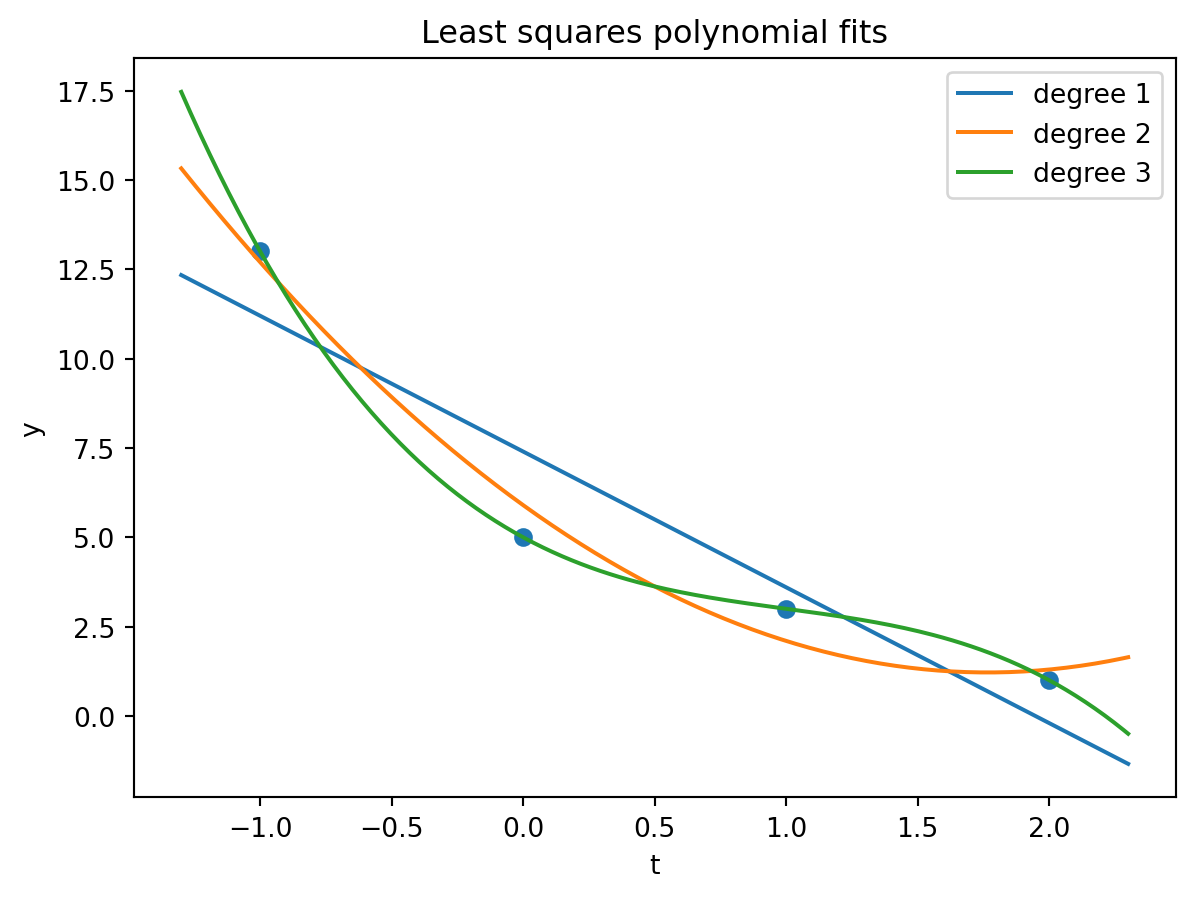
### Example 12.16: Cubic interpolation
Find a cubic polynomial
$$
f(t)=c_0+c_1t+c_2t^2+c_3t^3
$$
passing through
$$
(0,5),\quad (1,3),\quad (-1,13),\quad (2,1).
$$
The linear system is
$$
\begin{bmatrix}
1&0&0&0\\
1&1&1&1\\
1&-1&1&-1\\
1&2&4&8
\end{bmatrix}
\begin{bmatrix}c_0\\c_1\\c_2\\c_3\end{bmatrix}
=
\begin{bmatrix}5\\3\\13\\1\end{bmatrix}.
$$
Solving gives
$$
\begin{bmatrix}c_0\\c_1\\c_2\\c_3\end{bmatrix}
=
\begin{bmatrix}5\\-4\\3\\-1\end{bmatrix},
$$
so
$$
f(t)=5-4t+3t^2-t^3.
$$
### Example 12.17: Quadratic least squares fit
Fit
$$
g(t)=c_0+c_1t+c_2t^2
$$
to the same four points. The design matrix is
$$
A=
\begin{bmatrix}
1&0&0\\
1&1&1\\
1&-1&1\\
1&2&4
\end{bmatrix},
\qquad
\vec{b}=\begin{bmatrix}5\\3\\13\\1\end{bmatrix}.
$$
The normal equations give
$$
\vec{c}=\begin{bmatrix}29/5\\-16/5\\3/5\end{bmatrix}.
$$
Hence
$$
g(t)=\frac{29}{5}-\frac{16}{5}t+\frac35t^2.
$$
### Example 12.18: Linear least squares fit
Fit
$$
h(t)=c_0+c_1t
$$
to the same four points. Then
$$
A=
\begin{bmatrix}
1&0\\
1&1\\
1&-1\\
1&2
\end{bmatrix},
\qquad
\vec{b}=\begin{bmatrix}5\\3\\13\\1\end{bmatrix}.
$$
Solving the normal equations gives
$$
\vec{c}=\begin{bmatrix}37/6\\-61/18\end{bmatrix}.
$$
Thus
$$
h(t)=\frac{37}{6}-\frac{61}{18}t.
$$
### Python visualization
```{python}
import matplotlib.pyplot as plt

t = np.array([0, 1, -1, 2], dtype=float)
y = np.array([5, 3, 13, 1], dtype=float)

for degree in [1, 2, 3]:
    A = np.vander(t, N=degree+1, increasing=True)
    coeff = np.linalg.lstsq(A, y, rcond=None)[0]
    grid = np.linspace(-1.3, 2.3, 200)
    G = np.vander(grid, N=degree+1, increasing=True)
    plt.plot(grid, G @ coeff, label=f"degree {degree}")

plt.scatter(t, y)
plt.xlabel("t")
plt.ylabel("y")
plt.legend()
plt.title("Least squares polynomial fits")
plt.show()
```
## 12.9 General regression models
### Simple linear regression
Given data
$$
(a_1,b_1),\ldots,(a_n,b_n),
$$
fit
$$
h(t)=c_0+c_1t.
$$
The design matrix and target vector are
$$
A=
\begin{bmatrix}
1&a_1\\
1&a_2\\
\vdots&\vdots\\
1&a_n
\end{bmatrix},
\qquad
\vec{b}=\begin{bmatrix}b_1\\b_2\\\vdots\\b_n\end{bmatrix}.
$$
The normal equations are
$$
\begin{bmatrix}
n&\sum a_i\\
\sum a_i&\sum a_i^2
\end{bmatrix}
\begin{bmatrix}c_0\\c_1\end{bmatrix}
=
\begin{bmatrix}\sum b_i\\\sum a_i b_i\end{bmatrix}.
$$
### Multiple linear regression
For inputs $(a_{i1},\ldots,a_{im})$ and outputs $b_i$, fit
$$
h(t_1,\ldots,t_m)=c_0+c_1t_1+\cdots+c_mt_m.
$$
Use
$$
A=
\begin{bmatrix}
1&a_{11}&\cdots&a_{1m}\\
1&a_{21}&\cdots&a_{2m}\\
\vdots&\vdots&\ddots&\vdots\\
1&a_{n1}&\cdots&a_{nm}
\end{bmatrix}.
$$
Then solve
$$
A^TA\vec{c}=A^T\vec{b}.
$$
### Multiple outputs
If the outputs form a matrix $B$, then the least squares matrix problem is
$$
AX\approx B.
$$
The normal equations are
$$
A^TAX=A^TB.
$$
If $A$ has full column rank,
$$
X=(A^TA)^{-1}A^TB.
$$
## 12.10 Best approximation of functions
Let $V=C[0,1]$ with inner product
$$
\langle f,g\rangle=\int_0^1 f(x)g(x)\,dx.
$$
Let
$$
P_n=\operatorname{span}\{1,x,x^2,\ldots,x^n\}.
$$
The best degree-$n$ polynomial approximation to $f$ is
$$
p^*=\operatorname{proj}_{P_n}f.
$$
If
$$
p^*(x)=c_0+c_1x+\cdots+c_nx^n,
$$
then the residual $f-p^*$ is orthogonal to $P_n$:
$$
\langle f-p^*,x^k\rangle=0,
\qquad k=0,1,\ldots,n.
$$
Thus
$$
\sum_{j=0}^n c_j\int_0^1 x^{j+k}\,dx
=
\int_0^1 f(x)x^k\,dx.
$$
Since
$$
\int_0^1 x^{j+k}\,dx=\frac{1}{j+k+1},
$$
the coefficient matrix is a Hilbert matrix.
### Example 12.19: Best linear approximation of $e^x$
Find the best approximation to $f(x)=e^x$ in $P_1=\operatorname{span}\{1,x\}$.
Write
$$
p(x)=c_0+c_1x.
$$
The normal equations are
$$
\begin{bmatrix}
1&1/2\\
1/2&1/3
\end{bmatrix}
\begin{bmatrix}c_0\\c_1\end{bmatrix}
=
\begin{bmatrix}e-1\\1\end{bmatrix}.
$$
Solving gives
$$
c_0=4e-10,
\qquad
c_1=18-6e.
$$
Therefore
$$
p(x)=(4e-10)+(18-6e)x.
$$
## 12.11 AI companion activities
These activities are designed to help you use AI as a study partner, not as a substitute for your own reasoning.
### Activity A: Explain the geometry
Ask an AI tool:
> Explain why the least squares solution of $A\vec{x}=\vec{b}$ is a projection onto $\operatorname{Col}(A)$, using a picture in words.
Then check whether the explanation includes the residual condition
$$
\vec{b}-A\vec{x}^{\,*}\perp \operatorname{Col}(A).
$$
### Activity B: Debug a normal-equation computation
Give an AI tool a matrix $A$ and vector $\vec{b}$ and ask it to compute $A^TA$ and $A^T\vec{b}$. Verify the answer using Python.
### Activity C: Compare methods
Ask:
> Why is QR factorization often more stable than solving least squares by normal equations?
A good answer should mention that forming $A^TA$ can square the condition number.
### Activity D: Create a data-fitting example
Ask AI to generate five noisy data points from a line. Then use Python to compute the least squares fit and compare the recovered line to the original line.
## 12.12 Classical challenge questions
### Challenge 1: Why the residual is unique
Suppose $A\vec{x}=\vec{b}$ has many least squares solutions. Prove that the fitted vector $A\vec{x}^{\,*}$ and residual $\vec{b}-A\vec{x}^{\,*}$ are unique.
<details>
<summary><strong>Show solution</strong></summary>
Every least squares solution satisfies
$$
A\vec{x}^{\,*}=\operatorname{proj}_{\operatorname{Col}(A)}\vec{b}.
$$
The orthogonal projection is unique. Hence the fitted vector is unique. The residual is
$$
\vec{b}-A\vec{x}^{\,*},
$$
so it is also unique.
</details>
### Challenge 2: Normal equations as an optimization condition
Let
$$
F(\vec{x})=\|A\vec{x}-\vec{b}\|^2.
$$
Show that $\nabla F(\vec{x})=0$ gives the normal equations.
<details>
<summary><strong>Show solution</strong></summary>
Expand:
$$
F(\vec{x})=(A\vec{x}-\vec{b})^T(A\vec{x}-\vec{b})
=\vec{x}^{\,T}A^TA\vec{x}-2\vec{x}^{\,T}A^T\vec{b}+\vec{b}^{\,T}\vec{b}.
$$
Taking the gradient gives
$$
\nabla F(\vec{x})=2A^TA\vec{x}-2A^T\vec{b}.
$$
Setting this equal to zero gives
$$
A^TA\vec{x}=A^T\vec{b}.
$$
</details>
### Challenge 3: Weighted least squares by optimization
Let $W$ be symmetric positive definite and define
$$
F_W(\vec{x})=(A\vec{x}-\vec{b})^TW(A\vec{x}-\vec{b}).
$$
Show that the critical point satisfies $A^TWA\vec{x}=A^TW\vec{b}$.
<details>
<summary><strong>Show solution</strong></summary>
Expanding gives
$$
F_W(\vec{x})=\vec{x}^{\,T}A^TWA\vec{x}-2\vec{x}^{\,T}A^TW\vec{b}+\vec{b}^{\,T}W\vec{b}.
$$
Because $W$ is symmetric,
$$
\nabla F_W(\vec{x})=2A^TWA\vec{x}-2A^TW\vec{b}.
$$
Setting the gradient equal to zero gives
$$
A^TWA\vec{x}=A^TW\vec{b}.
$$
</details>
## 12.13 Practice problems
### Problem 1
Let
$$
A=\begin{bmatrix}1\\1\\1\end{bmatrix},
\qquad
\vec{b}=\begin{bmatrix}2\\4\\5\end{bmatrix}.
$$
Find the least squares solution and interpret it.
<details>
<summary><strong>Show solution</strong></summary>
The normal equation is
$$
3x=11.
$$
Thus
$$
x=\frac{11}{3}.
$$
This is the average of the observations $2,4,5$. The fitted vector is
$$
Ax=\begin{bmatrix}11/3\\11/3\\11/3\end{bmatrix}.
$$
</details>
### Problem 2
Let
$$
A=\begin{bmatrix}1&0\\1&1\\1&2\end{bmatrix},
\qquad
\vec{b}=\begin{bmatrix}1\\2\\4\end{bmatrix}.
$$
Find the least squares line $h(t)=c_0+c_1t$.
<details>
<summary><strong>Show solution</strong></summary>
Compute
$$
A^TA=\begin{bmatrix}3&3\\3&5\end{bmatrix},
\qquad
A^T\vec{b}=\begin{bmatrix}7\\10\end{bmatrix}.
$$
Solving gives
$$
\vec{c}=\begin{bmatrix}5/6\\3/2\end{bmatrix}.
$$
Therefore
$$
h(t)=\frac56+\frac32t.
$$
</details>
### Problem 3
For
$$
A=\begin{bmatrix}1&1\\1&1\\1&1\end{bmatrix},
\qquad
\vec{b}=\begin{bmatrix}1\\2\\3\end{bmatrix},
$$
find all least squares solutions.
<details>
<summary><strong>Show solution</strong></summary>
The normal equations reduce to
$$
x_1+x_2=2.
$$
Therefore all least squares solutions are
$$
\vec{x}^{\,*}=\begin{bmatrix}t\\2-t\end{bmatrix},
\qquad t\in\mathbb{R}.
$$
The fitted vector is always
$$
\begin{bmatrix}2\\2\\2\end{bmatrix}.
$$
</details>
### Problem 4
Set up the normal equations for the best quadratic approximation to $f(x)=\sin x$ on $[0,1]$.
<details>
<summary><strong>Show solution</strong></summary>
Let
$$
p(x)=c_0+c_1x+c_2x^2.
$$
The normal equations are
$$
\int_0^1(\sin x-p(x))x^k\,dx=0,
\qquad k=0,1,2.
$$
Equivalently,
$$
\sum_{j=0}^2 c_j\int_0^1 x^{j+k}\,dx
=
\int_0^1 x^k\sin x\,dx,
\qquad k=0,1,2.
$$
</details>
### Problem 5
Explain why $A^TA$ is invertible if the columns of $A$ are linearly independent.
<details>
<summary><strong>Show solution</strong></summary>
If the columns of $A$ are linearly independent, then $\ker(A)=\{0\}$. Since $\ker(A)=\ker(A^TA)$, we also have $\ker(A^TA)=\{0\}$. The matrix $A^TA$ is square, so trivial kernel implies invertibility.
</details>