3  Chapter 3. The Many Homes of Vectors: Spaces, Subspaces, and Linear Maps

From columns to functions, polynomials, matrices, quotients, and tensors

Guiding question.
What is the same about column vectors, polynomials, functions, matrices, and signals?

In Chapter 1, a matrix was a machine for organizing and solving linear systems. In Chapter 2, vectors became objects we could add, scale, combine, and visualize.

This chapter takes the next step. A vector does not have to be a column of numbers. A vector can be a polynomial. A vector can be a function. A vector can be a matrix. A vector can even be a linear transformation.

The central idea is simple:

A vector space is a world in which addition and scalar multiplication behave correctly.

Once we know we are in such a world, the same language works everywhere: subspaces, spans, direct sums, linear maps, kernels, images, quotient spaces, matrices, and tensor products.

NoteHow to read this chapter

This chapter keeps a story-driven style, but the definitions and theorems are precise. The goal is to help you move among three viewpoints:

1. concrete computation: solve systems, find spans, compute kernels;
2. geometric structure: lines, planes, subspaces, quotient spaces;
3. abstract transfer: use the same ideas for functions, polynomials, matrices, and data.

TipAI and coding companion

Use Python, MATLAB, or AI tools to check examples, but keep the mathematical questions precise. For example, instead of asking “solve this,” ask:

Find a basis for the kernel, find a basis for the image, and explain why the dimensions are consistent.

3.1 3.1 The idea of a linear space

The word vector often brings to mind an arrow or a column such as

\[ \begin{bmatrix}2\\-1\\4\end{bmatrix}. \]

But linear algebra is more flexible. The important question is not “Is this object drawn as an arrow?” The important question is:

Can we add two such objects, and can we multiply one by a scalar, while staying in the same collection?

NoteDefinition 3.1: Vector space

Let \(\mathbb F\) be a field. A vector space, or linear space, over \(\mathbb F\) is a nonempty set \(V\) together with two operations:

1. vector addition: for \(u,v\in V\), the sum \(u+v\in V\);
2. scalar multiplication: for \(c\in\mathbb F\) and \(u\in V\), the scalar multiple \(cu\in V\).

These operations satisfy the following axioms for all \(u,v,w\in V\) and all \(a,b\in\mathbb F\):

\[ \begin{aligned} u+v &= v+u,\\ (u+v)+w &= u+(v+w),\\ u+0 &= u,\\ u+(-u)&=0,\\ a(u+v)&=au+av,\\ (a+b)u&=au+bu,\\ a(bu)&=(ab)u,\\ 1u&=u. \end{aligned} \]

The elements of \(V\) are called vectors, even if they are functions, polynomials, matrices, or transformations.

The axioms look long, but the message is short: addition and scaling must behave the way they do in \(\mathbb R^n\).

ImportantProposition 3.2: Basic consequences

In every vector space \(V\) over \(\mathbb F\),

\[ 0u=0,\qquad c0=0,\qquad (-1)u=-u. \]

The zero vector is unique, and the additive inverse of each vector is unique.

NoteProof idea

For example, since \(0=0+0\) in the field,

\[ 0u=(0+0)u=0u+0u. \]

Add the inverse of \(0u\) to both sides to get \(0=0u\). The other identities are similar consequences of the axioms.

3.1.1 Standard examples

TipExamples 3.3: Many homes of vectors

Each of the following is a vector space with the natural addition and scalar multiplication:

1. coordinate space \(\mathbb F^n\);
2. matrix space \(\mathbb F^{m\times n}\);
3. polynomial space \(\mathbb F[t]\);
4. polynomial space \(\mathbb F_n[t]\) of degree at most \(n\);
5. function space \(\{f:X\to\mathbb F\}\);
6. continuous functions \(C([0,1])\);
7. solutions of a homogeneous linear differential equation, such as \(y''+y=0\).

The last example is important. If \(y_1\) and \(y_2\) both satisfy \(y''+y=0\), then every linear combination

\[ cy_1+dy_2 \]

also satisfies the same equation. That is why homogeneous linear differential equations belong naturally to linear algebra.

3.1.2 A function-space example

Let

\[ V=C([0,1]),\qquad f(t)=e^t,\qquad g(t)=\sin(\pi t). \]

For \(a,b\in\mathbb R\),

\[ h(t)=af(t)+bg(t)=ae^t+b\sin(\pi t) \]

is still continuous on \([0,1]\). Thus \(h\in V\). Once we know \(C([0,1])\) is a vector space, we can talk about spans, subspaces, linear transformations, kernels, and images in this infinite collection of functions.

3.2 3.2 Nonexamples: how vector spaces fail

To show that a set is not a vector space, we only need to find one failed rule. The most common failures are:

1. the zero vector is missing;
2. the set is not closed under addition;
3. the set is not closed under scalar multiplication.

CautionExample 3.4: Degree exactly three is not a vector space

The set

\[ H=\{p(t)\in\mathbb R[t]:\deg p=3\} \]

is not a vector space. It does not contain the zero polynomial. It is also not closed under addition. For example,

\[ (t^3+1)+(-t^3+t)=t+1, \]

which has degree \(1\), not degree \(3\).

CautionExample 3.5: Affine constraints usually fail

The set

\[ H=\{(x_1,x_2)\in\mathbb R^2:2x_1-x_2=1\} \]

is not a vector space because \((0,0)\notin H\).

The related homogeneous set

\[ L=\{(x_1,x_2)\in\mathbb R^2:2x_1-x_2=0\} \]

is a vector space. Geometrically, \(H\) is a shifted line, while \(L\) is a line through the origin.

3.3 3.3 Subspaces: smaller linear worlds

A subspace is a vector space inside another vector space.

NoteDefinition 3.6: Subspace

Let \(V\) be a vector space over \(\mathbb F\). A subset \(U\subseteq V\) is a subspace of \(V\) if:

1. \(0\in U\);
2. if \(u,v\in U\), then \(u+v\in U\);
3. if \(u\in U\) and \(c\in\mathbb F\), then \(cu\in U\).

ImportantTheorem 3.7: Subspace theorem

If \(U\) is a subspace of a vector space \(V\), then \(U\) is itself a vector space using the addition and scalar multiplication inherited from \(V\).

The subspace theorem is a time saver. We do not check all eight vector-space axioms again. We only check zero, addition, and scalar multiplication.

3.3.1 Polynomial subspaces

Let

\[ \mathbb R_4[t]=\{a_0+a_1t+a_2t^2+a_3t^3+a_4t^4:a_i\in\mathbb R\}. \]

This is a subspace of \(\mathbb R[t]\).

Now consider

\[ H=\{at^4+b:a,b\in\mathbb R\}\subseteq \mathbb R_4[t]. \]

Then \(H\) is also a subspace because

\[ (at^4+b)+(ct^4+d)=(a+c)t^4+(b+d) \]

and

\[ \lambda(at^4+b)=(\lambda a)t^4+\lambda b. \]

3.3.2 Matrix subspaces

The following are subspaces of \(\mathbb R^{n\times n}\):

1. upper triangular matrices;
2. lower triangular matrices;
3. diagonal matrices;
4. symmetric matrices;
5. skew-symmetric matrices.

For example, if \(A^T=A\) and \(B^T=B\), then

\[ (A+B)^T=A^T+B^T=A+B, \]

so \(A+B\) is symmetric. Also,

\[ (cA)^T=cA^T=cA. \]

Thus the symmetric matrices form a subspace.

CautionExample 3.8: Invertible matrices are not a subspace

The set of invertible \(n\times n\) matrices is not a subspace of \(\mathbb R^{n\times n}\). It does not contain the zero matrix. It is also not closed under addition, because \(I\) and \(-I\) are invertible, but

\[ I+(-I)=0 \]

is not invertible.

3.3.3 Geometric subspaces

The set

\[ U=\{(x_1,x_2,x_3)\in\mathbb R^3:3x_1-5x_2+x_3=0\} \]

is a subspace of \(\mathbb R^3\). It is the solution set of a homogeneous linear equation. Equivalently,

\[ U=\ker A, \qquad A=\begin{bmatrix}3&-5&1\end{bmatrix}. \]

Kernels of linear maps are always subspaces.

By contrast,

\[ C=\{(x_1,x_2)\in\mathbb R^2:x_1\ge 0,\ x_2\ge 0\} \]

is not a subspace. It is closed under addition and nonnegative scaling, but not under multiplication by negative scalars.

3.4 3.4 Span: building subspaces from vectors

The span of vectors is the set of all linear combinations of those vectors.

NoteDefinition 3.9: Linear combination and span

Let \(v_1,\ldots,v_m\in V\). A linear combination of these vectors is a vector of the form

\[ c_1v_1+c_2v_2+\cdots+c_mv_m, \qquad c_i\in\mathbb F. \]

The span is

\[ \operatorname{span}(v_1,\ldots,v_m) = \{c_1v_1+\cdots+c_mv_m:c_i\in\mathbb F\}. \]

ImportantTheorem 3.10: Span is a subspace

For any vectors \(v_1,\ldots,v_m\in V\), the set \(\operatorname{span}(v_1,\ldots,v_m)\) is a subspace of \(V\).

NoteProof idea

The zero vector is obtained by taking all coefficients equal to zero. The sum of two linear combinations is another linear combination. A scalar multiple of a linear combination is also another linear combination.

3.4.1 A plane as a span

Let

\[ u_1=(1,0,2),\qquad u_2=(0,1,-1). \]

Then

\[ \operatorname{span}(u_1,u_2) = \{s(1,0,2)+t(0,1,-1):s,t\in\mathbb R\} = \{(s,t,2s-t):s,t\in\mathbb R\}. \]

This is a plane through the origin. Since \(x_1=s\), \(x_2=t\), and \(x_3=2s-t\), the equation of the plane is

\[ 2x_1-x_2-x_3=0. \]

3.4.2 Polynomial span and membership

In \(\mathbb R_3[t]\), let

\[ p_1(t)=1+t,\qquad p_2(t)=t+t^2,\qquad p_3(t)=t^2+t^3. \]

A general linear combination is

\[ a(1+t)+b(t+t^2)+c(t^2+t^3) =a+(a+b)t+(b+c)t^2+ct^3. \]

So a polynomial

\[ \alpha+\beta t+\gamma t^2+\delta t^3 \]

belongs to the span exactly when there are \(a,b,c\) satisfying

\[ a=\alpha,\qquad a+b=\beta,\qquad b+c=\gamma,\qquad c=\delta. \]

Eliminating \(a,b,c\) gives

\[ \gamma=\beta-\alpha+\delta. \]

Thus span questions are often hidden linear-system questions.

3.5 3.5 Sums and direct sums

Sometimes a vector space is built from two smaller subspaces.

NoteDefinition 3.11: Sum of subspaces

Let \(U\) and \(W\) be subspaces of \(V\). Their sum is

\[ U+W=\{u+w:u\in U,\ w\in W\}. \]

ImportantProposition 3.12: Sum is a subspace

If \(U\) and \(W\) are subspaces of \(V\), then \(U+W\) is a subspace of \(V\).

NoteDefinition 3.13: Direct sum

We say that \(V\) is the direct sum of \(U\) and \(W\), written

\[ V=U\oplus W, \]

if every vector \(v\in V\) can be written uniquely as

\[ v=u+w, \qquad u\in U,\quad w\in W. \]

ImportantTheorem 3.14: Direct-sum test

Let \(U\) and \(W\) be subspaces of \(V\). Then

\[ V=U\oplus W \]

if and only if

\[ V=U+W \qquad\text{and}\qquad U\cap W=\{0\}. \]

3.5.1 Direct sum in \(\mathbb R^3\)

Let

\[ U=\{(x,0,0):x\in\mathbb R\}, \qquad W=\{(0,y,z):y,z\in\mathbb R\}. \]

Then every vector \((a,b,c)\in\mathbb R^3\) decomposes as

\[ (a,b,c)=(a,0,0)+(0,b,c). \]

Also \(U\cap W=\{(0,0,0)\}\). Hence

\[ \mathbb R^3=U\oplus W. \]

3.5.2 A sum that is not direct

Let

\[ U=\{(x,y,0):x,y\in\mathbb R\}, \qquad W=\{(0,y,z):y,z\in\mathbb R\}. \]

Then \(U+W=\mathbb R^3\), but

\[ U\cap W=\{(0,y,0):y\in\mathbb R\}\ne\{0\}. \]

So the decomposition is not unique. For example,

\[ (1,2,3)=(1,0,0)+(0,2,3)=(1,5,0)+(0,-3,3). \]

3.5.3 Symmetric and skew-symmetric matrices

Let

\[ \operatorname{Sym}_n=\{A\in\mathbb R^{n\times n}:A^T=A\}, \qquad \operatorname{Skew}_n=\{A\in\mathbb R^{n\times n}:A^T=-A\}. \]

Every matrix \(A\in\mathbb R^{n\times n}\) has the decomposition

\[ A=\frac{A+A^T}{2}+\frac{A-A^T}{2}. \]

The first term is symmetric, and the second term is skew-symmetric. Their intersection is \(\{0\}\). Therefore

\[ \mathbb R^{n\times n}=\operatorname{Sym}_n\oplus \operatorname{Skew}_n. \]

This example is important because it decomposes a matrix space into two natural subspaces.

3.6 3.6 Linear transformations

A linear transformation is a function that respects the linear structure.

NoteDefinition 3.15: Linear transformation

Let \(V\) and \(W\) be vector spaces over \(\mathbb F\). A function

\[ T:V\to W \]

is linear if, for all \(u,v\in V\) and all \(c\in\mathbb F\),

\[ T(u+v)=T(u)+T(v), \qquad T(cu)=cT(u). \]

ImportantProposition 3.16: Linear maps preserve linear combinations

If \(T:V\to W\) is linear, then

\[ T(c_1v_1+\cdots+c_kv_k) = c_1T(v_1)+\cdots+c_kT(v_k). \]

In particular, \(T(0)=0\).

3.6.1 Examples of linear transformations

Differentiation. The derivative map

\[ D:\mathbb R_n[t]\to\mathbb R_{n-1}[t], \qquad D(p)=p' \]

is linear because

\[ D(ap+bq)=aD(p)+bD(q). \]

For example, if \(p(t)=3t^4-2t+1\), then

\[ D(p)=12t^3-2. \]

Trace. The trace map

\[ \operatorname{tr}:\mathbb R^{n\times n}\to\mathbb R, \qquad \operatorname{tr}(A)=a_{11}+\cdots+a_{nn} \]

is linear.

Evaluation. For \(V=C([0,1])\), the evaluation map

\[ E_{1/2}:V\to\mathbb R, \qquad E_{1/2}(f)=f(1/2) \]

is linear.

A nonlinear map. The map

\[ T:\mathbb R^n\to\mathbb R, \qquad T(x)=\|x\|^2 \]

is not linear because

\[ T(cx)=\|cx\|^2=c^2\|x\|^2, \]

which is usually not equal to \(cT(x)\).

3.7 3.7 Kernel, image, injectivity, and surjectivity

Linear maps are understood by two fundamental subspaces: the kernel and the image.

NoteDefinition 3.17: Kernel and image

Let \(T:V\to W\) be a linear transformation. The kernel of \(T\) is

\[ \ker(T)=\{v\in V:T(v)=0\}. \]

The image, or range, of \(T\) is

\[ \operatorname{im}(T)=\{T(v):v\in V\}\subseteq W. \]

ImportantTheorem 3.18: Kernel and image are subspaces

If \(T:V\to W\) is linear, then \(\ker(T)\) is a subspace of \(V\) and \(\operatorname{im}(T)\) is a subspace of \(W\).

ImportantTheorem 3.19: Injectivity and surjectivity tests

Let \(T:V\to W\) be linear.

1. \(T\) is injective if and only if \(\ker(T)=\{0\}\).
2. \(T\) is surjective if and only if \(\operatorname{im}(T)=W\).

NoteDefinition 3.20: Isomorphism

Two vector spaces \(V\) and \(W\) are isomorphic, written \(V\cong W\), if there exists an invertible linear transformation

\[ T:V\to W. \]

An isomorphism means that \(V\) and \(W\) have the same linear structure, even if their elements look different.

3.7.1 Kernel and image of differentiation

Let

\[ D:\mathbb R_3[t]\to\mathbb R_2[t], \qquad D(p)=p'. \]

If

\[ p(t)=a+bt+ct^2+dt^3, \]

then

\[ D(p)=b+2ct+3dt^2. \]

Therefore

\[ \ker(D)=\{a:a\in\mathbb R\}=\operatorname{span}(1), \]

and

\[ \operatorname{im}(D)=\mathbb R_2[t]. \]

So \(D\) is surjective but not injective.

3.7.2 A linear functional on \(\mathbb R^3\)

Let

\[ T:\mathbb R^3\to\mathbb R, \qquad T(x,y,z)=2x-y+3z. \]

Then

\[ \ker(T)=\{(x,y,z):2x-y+3z=0\}, \]

a plane through the origin. Since \(T(1/2,0,0)=1\), the image contains \(1\), so

\[ \operatorname{im}(T)=\mathbb R. \]

Thus \(T\) is surjective but not injective.

3.7.3 Finding a transformation with a prescribed kernel

Suppose we want a linear transformation whose kernel is the plane

\[ 2x-y+3z=0. \]

Use the linear functional

\[ T(x,y,z)=2x-y+3z. \]

Then \(\ker(T)\) is exactly the given plane. Any nonzero scalar multiple

\[ T_c(x,y,z)=c(2x-y+3z),\qquad c\ne 0, \]

has the same kernel.

3.8 3.8 Computing kernel and image from a matrix

Let \(T:\mathbb R^4\to\mathbb R^3\) be defined by \(T(x)=Ax\), where

\[ A= \begin{bmatrix} 0&0&2&8\\ 1&5&2&-5\\ 2&10&6&-2 \end{bmatrix}. \]

A row reduction gives

\[ \operatorname{rref}(A)= \begin{bmatrix} 1&5&0&-13\\ 0&0&1&4\\ 0&0&0&0 \end{bmatrix}. \]

The pivot columns are columns \(1\) and \(3\). Therefore

\[ \operatorname{im}(T)= \operatorname{span}\left\{ \begin{bmatrix}0\\1\\2\end{bmatrix}, \begin{bmatrix}2\\2\\6\end{bmatrix} \right\}. \]

To find the kernel, solve \(Ax=0\). From the rref matrix,

\[ x_1=-5x_2+13x_4, \qquad x_3=-4x_4. \]

Thus

\[ x=x_2\begin{bmatrix}-5\\1\\0\\0\end{bmatrix} +x_4\begin{bmatrix}13\\0\\-4\\1\end{bmatrix}. \]

So

\[ \ker(T)= \operatorname{span}\left\{ \begin{bmatrix}-5\\1\\0\\0\end{bmatrix}, \begin{bmatrix}13\\0\\-4\\1\end{bmatrix} \right\}. \]

TipComputation principle

For a matrix transformation \(T(x)=Ax\):

1. the image is the column space of \(A\);
2. a basis for the image comes from pivot columns of the original matrix;
3. the kernel is the solution set of \(Ax=0\);
4. the free variables give a basis for the kernel.

3.9 3.9 Linear maps as a vector space and the dual space

A surprising but powerful idea is that linear maps themselves can be vectors.

NoteDefinition 3.21: Space of linear maps

Let \(V\) and \(W\) be vector spaces over \(\mathbb F\). Denote by

\[ \mathcal L(V,W) \]

the set of all linear transformations from \(V\) to \(W\).

ImportantTheorem 3.22: Linear maps form a vector space

The set \(\mathcal L(V,W)\) is a vector space under pointwise operations:

\[ (S+T)(v)=S(v)+T(v), \qquad (cT)(v)=cT(v). \]

NoteDefinition 3.23: Dual space

The dual space of \(V\) is

\[ V^*=\mathcal L(V,\mathbb F). \]

Its elements are called linear functionals.

A linear functional is a linear measurement. It takes a vector and returns one scalar.

3.9.1 Dual vectors in \(\mathbb R^n\)

Every row vector \(a^T\in\mathbb R^{1\times n}\) defines a linear functional

\[ \varphi_a(x)=a^Tx. \]

For example, if \(a=(2,-1,3)\), then

\[ \varphi_a(x,y,z)=2x-y+3z. \]

3.9.2 Dual basis in a polynomial space

Let \(V=\mathbb R_2[t]\) with basis \((1,t,t^2)\). Define

\[ \varepsilon_0(p)=p(0), \qquad \varepsilon_1(p)=p'(0), \qquad \varepsilon_2(p)=\frac{p''(0)}{2}. \]

If

\[ p(t)=a+bt+ct^2, \]

then

\[ \varepsilon_0(p)=a, \qquad \varepsilon_1(p)=b, \qquad \varepsilon_2(p)=c. \]

These functionals recover the coordinates of \(p\) in the standard polynomial basis.

3.10 3.10 Quotient spaces: collapsing a subspace to zero

A quotient space identifies vectors that differ by a chosen subspace.

The guiding picture is this:

If \(N\) is information we decide to ignore, then \(V/N\) keeps only the information transverse to \(N\).

NoteDefinition 3.24: Equivalence relation from a subspace

Let \(N\) be a subspace of a vector space \(V\). Define

\[ v\sim w \qquad\text{if and only if}\qquad v-w\in N. \]

The equivalence class of \(v\) is the coset

\[ [v]=v+N=\{v+n:n\in N\}. \]

NoteDefinition 3.25: Quotient space

The quotient space \(V/N\) is the set of all cosets \(v+N\). Addition and scalar multiplication are defined by

\[ [v]+[w]=[v+w], \qquad c[v]=[cv]. \]

ImportantTheorem 3.26: Quotient space theorem

If \(N\) is a subspace of \(V\), then \(V/N\) is a vector space. The natural projection

\[ \pi:V\to V/N, \qquad \pi(v)=[v], \]

is linear and satisfies

\[ \ker(\pi)=N. \]

If \(V\) is finite-dimensional, then

\[ \dim(V/N)=\dim(V)-\dim(N). \]

3.10.1 Example: quotient of \(\mathbb R^2\) by the \(x\)-axis

Let

\[ V=\mathbb R^2, \qquad N=\operatorname{span}\{(1,0)\}. \]

Then two vectors \((x,y)\) and \((x',y')\) are equivalent if

\[ (x,y)-(x',y')=(x-x',y-y')\in N. \]

This happens exactly when \(y=y'\). Thus the quotient \(\mathbb R^2/N\) remembers only the vertical coordinate. Therefore

\[ \mathbb R^2/N\cong \mathbb R. \]

3.10.2 Quotient spaces and kernels

If \(T:V\to W\) is linear, then all vectors in a coset of \(\ker(T)\) have the same image. Indeed, if \(v-w\in\ker(T)\), then

\[ T(v-w)=0, \]

so

\[ T(v)=T(w). \]

This is the idea behind the first isomorphism theorem.

ImportantTheorem 3.27: First isomorphism theorem for vector spaces

Let \(T:V\to W\) be linear. Then

\[ V/\ker(T)\cong \operatorname{im}(T). \]

NoteProof idea

Define

\[ \Phi:V/\ker(T)\to \operatorname{im}(T), \qquad \Phi([v])=T(v). \]

This is well-defined because vectors in the same coset differ by an element of the kernel. The map is linear, injective, and surjective onto the image.

3.11 3.11 Linear transformations and matrices

Every matrix defines a linear transformation. Conversely, after choosing bases, every finite-dimensional linear transformation has a matrix.

NoteDefinition 3.28: Matrix representation

Let \(V\) and \(W\) be finite-dimensional vector spaces with ordered bases

\[ \mathcal B=(v_1,\ldots,v_n), \qquad \mathcal C=(w_1,\ldots,w_m). \]

For a linear map \(T:V\to W\), the matrix of \(T\) with respect to \(\mathcal B\) and \(\mathcal C\) is the matrix whose \(j\)-th column is the coordinate vector of \(T(v_j)\) in the basis \(\mathcal C\):

\[ [T]_{\mathcal C\leftarrow\mathcal B} = \begin{bmatrix} [T(v_1)]_{\mathcal C}&\cdots&[T(v_n)]_{\mathcal C} \end{bmatrix}. \]

The notation means: coordinates start in basis \(\mathcal B\) and land in basis \(\mathcal C\).

3.11.1 Example: derivative map as a matrix

Let

\[ D:\mathbb R_3[t]\to\mathbb R_2[t], \qquad D(p)=p'. \]

Use bases

\[ \mathcal B=(1,t,t^2,t^3), \qquad \mathcal C=(1,t,t^2). \]

Then

\[ D(1)=0, \qquad D(t)=1, \qquad D(t^2)=2t, \qquad D(t^3)=3t^2. \]

So

\[ [D]_{\mathcal C\leftarrow\mathcal B} = \begin{bmatrix} 0&1&0&0\\ 0&0&2&0\\ 0&0&0&3 \end{bmatrix}. \]

This matrix takes the coordinate vector of a polynomial in \(\mathbb R_3[t]\) and returns the coordinate vector of its derivative in \(\mathbb R_2[t]\).

3.12 3.12 Tensor products and Kronecker products

Tensor products give a systematic way to build new vector spaces from old ones.

NoteDefinition 3.29: Tensor product

Let \(V\) and \(W\) be vector spaces over \(\mathbb F\). The tensor product \(V\otimes W\) is a vector space generated by symbols

\[ v\otimes w, \qquad v\in V,\ w\in W, \]

subject to the bilinear rules

\[ (v_1+v_2)\otimes w=v_1\otimes w+v_2\otimes w, \]

\[ v\otimes(w_1+w_2)=v\otimes w_1+v\otimes w_2, \]

and

\[ (cv)\otimes w=v\otimes(cw)=c(v\otimes w). \]

ImportantTheorem 3.30: Basis and dimension of a tensor product

If \(\mathcal A=(a_1,\ldots,a_m)\) is a basis of \(V\) and \(\mathcal B=(b_1,\ldots,b_n)\) is a basis of \(W\), then

\[ \{a_i\otimes b_j:1\le i\le m,\ 1\le j\le n\} \]

is a basis of \(V\otimes W\). Therefore

\[ \dim(V\otimes W)=\dim(V)\dim(W). \]

3.12.1 Tensor product of coordinate spaces

There is a natural isomorphism

\[ \mathbb R^m\otimes\mathbb R^n\cong \mathbb R^{m\times n}. \]

A simple tensor \(v\otimes w\) corresponds to the rank-one matrix

\[ vw^T. \]

If

\[ v=\begin{bmatrix}v_1\\ \vdots\\ v_m\end{bmatrix}, \qquad w=\begin{bmatrix}w_1\\ \vdots\\ w_n\end{bmatrix}, \]

then

\[ v\otimes w \longleftrightarrow \begin{bmatrix} v_1w_1&\cdots&v_1w_n\\ \vdots&\ddots&\vdots\\ v_mw_1&\cdots&v_mw_n \end{bmatrix}. \]

3.12.2 Kronecker product

For matrices \(A=[a_{ij}]\in\mathbb R^{m\times n}\) and \(B\in\mathbb R^{p\times q}\), the Kronecker product is

\[ A\otimes B= \begin{bmatrix} a_{11}B&a_{12}B&\cdots&a_{1n}B\\ a_{21}B&a_{22}B&\cdots&a_{2n}B\\ \vdots&\vdots&\ddots&\vdots\\ a_{m1}B&a_{m2}B&\cdots&a_{mn}B \end{bmatrix} \in\mathbb R^{mp\times nq}. \]

This operation appears in numerical linear algebra, signal processing, quantum computing, graph products, and multidimensional data.

3.12.3 Example

Let

\[ A=\begin{bmatrix}1&2\\3&4\end{bmatrix}, \qquad B=\begin{bmatrix}0&5\\6&7\end{bmatrix}. \]

Then

\[ A\otimes B= \begin{bmatrix} 1B&2B\\ 3B&4B \end{bmatrix} = \begin{bmatrix} 0&5&0&10\\ 6&7&12&14\\ 0&15&0&20\\ 18&21&24&28 \end{bmatrix}. \]

3.13 3.13 Computation lab: subspaces and linear maps in Python

We now use Python to compute kernels, images, and Kronecker products.

import sympy as sp

A = sp.Matrix([
    [0, 0, 2, 8],
    [1, 5, 2, -5],
    [2, 10, 6, -2]
])

A_rref, pivots = A.rref()
A_rref, pivots

(Matrix([
 [1, 5, 0, -13],
 [0, 0, 1,   4],
 [0, 0, 0,   0]]),
 (0, 2))

The pivot columns are indexed from zero in Python. Therefore pivot indices (0, 2) mean columns \(1\) and \(3\) mathematically.

image_basis = A.columnspace()
kernel_basis = A.nullspace()

image_basis, kernel_basis

([Matrix([
  [0],
  [1],
  [2]]),
  Matrix([
  [2],
  [2],
  [6]])],
 [Matrix([
  [-5],
  [ 1],
  [ 0],
  [ 0]]),
  Matrix([
  [13],
  [ 0],
  [-4],
  [ 1]])])

3.13.1 Kronecker product in Python

A = sp.Matrix([[1, 2], [3, 4]])
B = sp.Matrix([[0, 5], [6, 7]])

sp.kronecker_product(A, B)

\(\displaystyle \left[\begin{matrix}0 & 5 & 0 & 10\\6 & 7 & 12 & 14\\0 & 15 & 0 & 20\\18 & 21 & 24 & 28\end{matrix}\right]\)

3.13.2 Visualizing a direct sum decomposition

The following code draws two coordinate subspaces in \(\mathbb R^3\): the \(x\)-axis and the \(yz\)-plane.

import numpy as np
import matplotlib.pyplot as plt

fig = plt.figure(figsize=(6, 5))
ax = fig.add_subplot(111, projection='3d')

# x-axis subspace U
x = np.linspace(-2, 2, 100)
ax.plot(x, 0*x, 0*x, label='U: x-axis')

# yz-plane subspace W
Y, Z = np.meshgrid(np.linspace(-2, 2, 10), np.linspace(-2, 2, 10))
X = np.zeros_like(Y)
ax.plot_surface(X, Y, Z, alpha=0.25)

# vector and decomposition
v = np.array([1.5, 1.0, 1.2])
u = np.array([1.5, 0.0, 0.0])
w = np.array([0.0, 1.0, 1.2])

ax.quiver(0, 0, 0, *v, length=1, normalize=False, label='v')
ax.quiver(0, 0, 0, *u, length=1, normalize=False, label='u in U')
ax.quiver(u[0], u[1], u[2], *w, length=1, normalize=False, label='w in W')

ax.set_xlabel('x')
ax.set_ylabel('y')
ax.set_zlabel('z')
ax.set_title(r'Direct sum $\mathbb{R}^3=U\oplus W$')
ax.legend()
plt.show()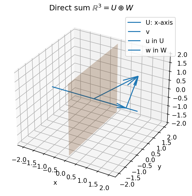

3.14 3.14 Chapter summary

This chapter expanded the meaning of vector beyond columns of numbers.

A vector space is any collection where addition and scalar multiplication behave correctly. A subspace is a smaller vector space inside a larger one. A span is the subspace generated by a list of vectors. A direct sum means every vector has a unique decomposition. A linear transformation is a structure-preserving map. Its kernel measures what collapses to zero, while its image measures what outputs are possible. The dual space consists of scalar-valued linear measurements. A quotient space collapses a subspace to zero. A matrix representation describes a linear transformation after bases are chosen. A tensor product builds larger vector spaces from smaller ones.

The main lesson is this:

Linear algebra is not only about solving systems. It is about recognizing structure that survives across many different kinds of mathematical objects.

3.15 3.15 Exercises

3.15.1 Conceptual exercises

1. Explain why \(\mathbb R_3[t]\) is a vector space but the set of polynomials of degree exactly \(3\) is not.

2. Give one example of a vector space whose elements are functions and one example whose elements are matrices.

3. Explain why a line in \(\mathbb R^2\) is a subspace if and only if it passes through the origin.

4. What is the difference between \(U+W\) and \(U\oplus W\)?

5. In your own words, explain what the kernel of a linear map measures.

3.15.2 Computational exercises

6. Determine whether each set is a subspace of the indicated vector space.

   1. \(\{(x,y,z)\in\mathbb R^3:x+y+z=0\}\) in \(\mathbb R^3\).

   2. \(\{(x,y,z)\in\mathbb R^3:x+y+z=1\}\) in \(\mathbb R^3\).

   3. \(\{A\in\mathbb R^{2\times 2}:\operatorname{tr}(A)=0\}\) in \(\mathbb R^{2\times 2}\).

7. Let

\[ u_1=(1,0,2),\qquad u_2=(0,1,-1). \]

Find an equation for \(\operatorname{span}(u_1,u_2)\).

8. Let

\[ T:\mathbb R^3\to\mathbb R, \qquad T(x,y,z)=x+2y-z. \]

Find \(\ker(T)\) and \(\operatorname{im}(T)\).

9. Let

\[ A=\begin{bmatrix} 1&2&3\\ 2&4&6\\ 1&1&1 \end{bmatrix}. \]

Find a basis for the column space and a basis for the null space.

10. Let \(D:\mathbb R_4[t]\to\mathbb R_3[t]\) be the derivative map. Find \(\ker(D)\) and \(\operatorname{im}(D)\).

11. Let \(V=\mathbb R^2\) and \(N=\operatorname{span}\{(1,1)\}\). Describe geometrically what the cosets in \(V/N\) look like.

12. Compute

\[ \begin{bmatrix}1&-1\\2&0\end{bmatrix} \otimes \begin{bmatrix}3&4\\5&6\end{bmatrix}. \]

3.15.3 Proof exercises

13. Prove that the intersection of two subspaces of \(V\) is a subspace of \(V\).

14. Prove that the sum \(U+W\) of two subspaces is a subspace.

15. Prove the direct-sum test: \(V=U\oplus W\) if and only if \(V=U+W\) and \(U\cap W=\{0\}\).

16. Prove that the kernel of a linear transformation is a subspace.

17. Prove that the image of a linear transformation is a subspace.

18. Prove that if \(T:V\to W\) is linear and injective, then \(T\) maps linearly independent sets to linearly independent sets.

3.15.4 Coding exercises

19. Use sympy to compute the rref, column space, and null space of the matrix in Exercise 9.

20. Write a Python function that takes a matrix \(A\) and returns rank(A), nullity(A), and verifies the rank-nullity formula.

21. Use Python to compute several Kronecker products and observe their sizes.

22. Use Python to represent the derivative map \(D:\mathbb R_4[t]\to\mathbb R_3[t]\) as a matrix.

3.15.5 AI companion exercises

23. Ask an AI tool: “Is every subset closed under addition a subspace?” Then critique the answer and give a counterexample.

24. Ask an AI tool to explain quotient spaces using \(\mathbb R^2\) modulo a line. Verify whether the explanation correctly identifies cosets.

25. Ask an AI tool to compute a kernel and image for a matrix. Then verify the result using row reduction.

3.16 Selected solutions

3.16.1 Solution to Exercise 6

1. The set is a subspace because it is the solution set of the homogeneous equation \(x+y+z=0\).

2. The set is not a subspace because \((0,0,0)\) does not satisfy \(x+y+z=1\).

3. The set is a subspace. The zero matrix has trace zero. Also,

\[ \operatorname{tr}(A+B)=\operatorname{tr}(A)+\operatorname{tr}(B) \]

and

\[ \operatorname{tr}(cA)=c\operatorname{tr}(A). \]

3.16.2 Solution to Exercise 7

A general vector in the span is

\[ s(1,0,2)+t(0,1,-1)=(s,t,2s-t). \]

Thus \(x=s\), \(y=t\), and \(z=2s-t=2x-y\). Therefore the equation is

\[ 2x-y-z=0. \]

3.16.3 Solution to Exercise 8

The kernel is

\[ \ker(T)=\{(x,y,z):x+2y-z=0\}. \]

Solving for \(x\) gives \(x=-2y+z\), so

\[ (x,y,z)=y(-2,1,0)+z(1,0,1). \]

Therefore

\[ \ker(T)=\operatorname{span}\{(-2,1,0),(1,0,1)\}. \]

Since \(T(1,0,0)=1\), the image contains \(1\), so

\[ \operatorname{im}(T)=\mathbb R. \]

3.16.4 Solution to Exercise 10

If

\[ p(t)=a+bt+ct^2+dt^3+et^4, \]

then

\[ D(p)=b+2ct+3dt^2+4et^3. \]

The kernel consists of constant polynomials, so

\[ \ker(D)=\operatorname{span}(1). \]

Every polynomial in \(\mathbb R_3[t]\) is the derivative of some polynomial in \(\mathbb R_4[t]\), so

\[ \operatorname{im}(D)=\mathbb R_3[t]. \]

3.16.5 Solution to Exercise 13

Let \(U\) and \(W\) be subspaces of \(V\). We prove \(U\cap W\) is a subspace.

First, \(0\in U\) and \(0\in W\), so \(0\in U\cap W\).

If \(a,b\in U\cap W\), then \(a,b\in U\) and \(a,b\in W\). Since \(U\) and \(W\) are subspaces, \(a+b\in U\) and \(a+b\in W\). Hence \(a+b\in U\cap W\).

If \(c\in\mathbb F\) and \(a\in U\cap W\), then \(a\in U\) and \(a\in W\). Since \(U\) and \(W\) are subspaces, \(ca\in U\) and \(ca\in W\). Hence \(ca\in U\cap W\).

Therefore \(U\cap W\) is a subspace.

3.16.6 Solution to Exercise 15

Assume \(V=U\oplus W\). Then every vector of \(V\) can be written as \(u+w\), so \(V=U+W\). If \(x\in U\cap W\), then

\[ 0=0+0=x+(-x), \]

where \(x\in U\) and \(-x\in W\). By uniqueness of decomposition, \(x=0\). Thus \(U\cap W=\{0\}\).

Conversely, assume \(V=U+W\) and \(U\cap W=\{0\}\). Since \(V=U+W\), every vector can be written as \(v=u+w\). Suppose

\[ u_1+w_1=u_2+w_2. \]

Then

\[ u_1-u_2=w_2-w_1. \]

The left side belongs to \(U\), and the right side belongs to \(W\). Therefore this vector belongs to \(U\cap W=\{0\}\). Hence \(u_1=u_2\) and \(w_1=w_2\). The decomposition is unique, so \(V=U\oplus W\).