Core idea: reinforcement learning is the mathematics of learning to make sequential decisions from interaction. The central object is not a labeled data set, but a stochastic feedback loop:
After reading this chapter, students should be able to:
describe the agent–environment interaction loop using state, action, reward, transition, and policy variables;
distinguish reinforcement learning from supervised learning, unsupervised learning, stochastic control, and dynamic programming;
define return, discounted return, state-value functions, and action-value functions;
explain why reinforcement learning data are usually not independent and identically distributed;
compute a value function in a small finite Markov reward model;
identify the mathematical themes that structure the rest of the book: conditional expectation, fixed points, stochastic approximation, optimization, and concentration.
4.2 1.1 The basic question
In supervised learning, the typical mathematical problem is to learn a function from examples:
\[
(x_i,y_i), \qquad i=1,\dots,n.
\]
The data are often modeled as independent samples from a fixed population distribution. The learner does not choose the data-generating process. It only chooses a predictor.
Reinforcement learning is different. The learner acts, and the action changes the future data distribution. A policy that explores one region of the state space produces one kind of data; a policy that avoids that region produces another. Thus the learner is simultaneously a statistician, an optimizer, and a controller.
A first informal definition is:
Reinforcement learning studies how an agent should choose actions over time in order to maximize long-run reward when the consequences of actions are stochastic and may be delayed.
This definition contains four mathematical ideas.
Phrase
Mathematical meaning
choose actions
optimization over policies
over time
stochastic process indexed by \(t\)
stochastic consequences
transition kernels and conditional distributions
delayed reward
dynamic programming and value functions
The modern field of reinforcement learning grew from several traditions: dynamic programming and optimal control (bellman1957dynamic?), Markov decision processes (puterman1994markov?), stochastic approximation, and machine learning (sutton2018reinforcement?).
4.3 1.2 The agent–environment loop
At each time step \(t=0,1,2,\dots\), an agent observes a state \(S_t\), chooses an action \(A_t\), receives a reward \(R_{t+1}\), and moves to a new state \(S_{t+1}\).
Here \(S\) is the state space and \(A(s)\) is the set of feasible actions at state \(s\). In a finite problem, \(S=\{1,\dots,m\}\) and each \(A(s)\) is a finite set. In continuous problems, states and actions may live in Euclidean spaces such as \(S\subseteq \mathbb R^d\) and \(A\subseteq \mathbb R^p\).
A trajectory has the form
\[
\tau=(S_0,A_0,R_1,S_1,A_1,R_2,S_2,\dots).
\]
The goal is not merely to predict the next state. The goal is to choose actions so that the entire trajectory is good according to a cumulative reward criterion.
4.3.1 Example 1.1: inventory control
Suppose \(S_t\) is the number of items in stock at the beginning of day \(t\). The action \(A_t\) is the number of new items to order. Random demand occurs during the day. The reward \(R_{t+1}\) may be negative total cost:
The action today changes tomorrow’s inventory. A greedy decision that minimizes today’s ordering cost may create large shortage cost later. This is the typical structure of reinforcement learning: immediate reward and future reward are coupled.
4.3.2 Example 1.2: treatment planning
Suppose \(S_t\) summarizes a patient’s current health information, \(A_t\) is a treatment decision, and \(R_{t+1}\) measures short-term clinical benefit minus side effects. The same treatment may help one patient state but harm another. Also, a treatment may have delayed consequences. This produces a sequential statistical decision problem.
4.3.3 Example 1.3: education and tutoring systems
Suppose \(S_t\) represents a student’s current knowledge state, \(A_t\) is the next learning activity, and \(R_{t+1}\) measures improvement, engagement, or mastery. The system must balance reviewing old material, introducing new concepts, and keeping the student engaged.
These examples look different, but mathematically they share the same feedback loop.
4.4 1.3 Policies
A policy is a rule for choosing actions. A deterministic policy is a function
\[
\pi:S\to A,
\]
where \(\pi(s)\) is the action chosen in state \(s\). A randomized policy assigns probabilities to actions:
where \(h_\theta(s,a)\) is a score function. The parameter vector \(\theta\) is learned from data.
4.5 1.4 Rewards, returns, and discounting
The reward \(R_{t+1}\) is the immediate numerical feedback after taking action \(A_t\) in state \(S_t\). However, the agent should usually care about more than the immediate reward.
These are conditional expectations. This point is essential for students from statistics: reinforcement learning is full of conditional expectations, but the conditioning events are produced by a policy that may change over time.
The optimal state-value function is
\[
V^*(s)=\sup_\pi V^\pi(s),
\]
and the optimal action-value function is
\[
Q^*(s,a)=\sup_\pi Q^\pi(s,a).
\]
A policy \(\pi^*\) is optimal if
\[
V^{\pi^*}(s)=V^*(s)
\qquad \text{for all } s\in S.
\]
The central computational problem is to find, approximate, or learn these functions.
4.7 1.6 Prediction, control, and learning
It is useful to separate three tasks.
Task
Question
Typical mathematical object
Prediction
How good is a fixed policy \(\pi\)?
\(V^\pi\), \(Q^\pi\)
Control
Which policy is best?
\(V^*\), \(Q^*\), \(\pi^*\)
Learning
How can we estimate or optimize from sampled experience?
Dynamic programming assumes that the transition law and reward model are known. Reinforcement learning usually assumes that at least part of the model is unknown and must be learned from samples.
This distinction produces a useful taxonomy.
Setting
Model known?
Data source
Representative methods
Dynamic programming
yes
exact transition and reward model
policy evaluation, policy iteration, value iteration
Monte Carlo RL
no
complete sampled episodes
sample averages of returns
Temporal-difference RL
no
one-step transitions
TD learning, SARSA, Q-learning
Approximate RL
no or partly
high-dimensional samples
linear approximation, neural networks
Offline RL
no
fixed historical data set
conservative and constrained learning
A mathematical book should not present these as unrelated algorithms. They are different approximations to related equations.
4.8 1.7 The Markov property
The most common model assumption in reinforcement learning is the Markov property. Informally, the current state contains all information needed for predicting the next state and reward, given the current action.
This does not mean that the past is irrelevant in a philosophical sense. It means the state variable \(S_t\) has been chosen so that past information relevant for future prediction is encoded in \(S_t\).
Modeling warning. The Markov property is not automatically true. It is a modeling assumption about the state representation. If important hidden variables are omitted, the process observed through \(S_t\) may fail to be Markov. This leads to partially observable Markov decision processes in Chapter 22.
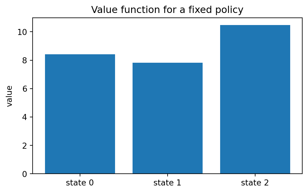
4.9 1.8 A first finite calculation
Consider a fixed policy in a small three-state system. Once the policy is fixed, the process behaves like a Markov reward process. Suppose the policy-induced transition matrix is
Second, the sampling distribution depends on the policy. If the policy changes, the distribution of future data changes.
This creates several statistical challenges.
Challenge
Meaning
dependence
samples along a trajectory are correlated
selection bias
the policy determines which states and actions are observed
exploration
good estimation may require trying uncertain actions
off-policy evaluation
data generated by one policy may be used to evaluate another
distribution shift
a learned policy may visit states rarely seen in the data
From a statistical point of view, reinforcement learning studies estimation and optimization under adaptive data collection.
4.11 1.10 Exploration versus exploitation
The agent faces a basic tension.
Exploitation: choose actions that currently seem best.
Exploration: choose actions to gain information that may improve future decisions.
A simple example is the multi-armed bandit problem. There is one state and several actions. Each action has an unknown reward distribution. Choosing an action gives a sample from its reward distribution, but only for the chosen action.
Let \(\mu_a=\mathbb E[R\mid A=a]\). If the means were known, the optimal action would be
\[
a^*\in \arg\max_a \mu_a.
\]
But the means are unknown. The agent must estimate them while also trying to collect reward. This is the simplest setting in which exploration matters.
A common exploratory policy is the \(\epsilon\)-greedy rule:
\[
A_t=
\begin{cases}
\arg\max_a \widehat Q_t(a), & \text{with probability } 1-\epsilon,\\
\text{a random action}, & \text{with probability } \epsilon.
\end{cases}
\]
Here \(\widehat Q_t(a)\) is the current estimate of action value. This rule is simple, but it introduces a theme that persists throughout the book: good learning requires both estimation and controlled experimentation.
4.12 1.11 Reinforcement learning as fixed-point computation
The Bellman equation is the mathematical center of reinforcement learning. In later chapters we will define Bellman operators precisely. For now, the important idea is this:
A value function is usually characterized as a fixed point of an operator.
For a fixed policy, the Bellman expectation operator has the form
Thus a large part of reinforcement learning can be understood as numerical fixed-point approximation.
Method
What it approximates
policy evaluation
fixed point of \(T^\pi\)
value iteration
fixed point of \(T^*\)
Monte Carlo prediction
conditional expectation defining \(V^\pi\)
TD learning
stochastic approximation to \(T^\pi V=V\)
Q-learning
stochastic approximation to optimal Bellman equation
policy gradient
gradient ascent on \(J(\theta)\)
4.13 1.12 Reinforcement learning as optimization
Another view is to start from a performance objective. For a parameterized policy \(\pi_\theta\), define
\[
J(\theta)=\mathbb E_{\pi_\theta}[G_0].
\]
The policy optimization problem is
\[
\max_\theta J(\theta).
\]
This looks like standard optimization, but there are two complications.
First, the expectation depends on \(\theta\) through the entire trajectory distribution. Changing \(\theta\) changes not just the action at one step, but the distribution of future states.
Second, \(J(\theta)\) is usually not available exactly. It must be estimated from sampled trajectories.
This gives rise to policy gradient methods, actor-critic algorithms, and modern deep reinforcement learning. These methods combine stochastic gradients with dynamic programming structure.
4.14 1.13 Relationship with neighboring fields
Reinforcement learning overlaps with several mathematical and statistical areas.
Field
Shared ideas
Difference in emphasis
Markov chains
transition matrices, stationarity, hitting times
RL includes actions and rewards
Dynamic programming
Bellman equations, optimal substructure
RL often learns from samples
Stochastic control
controlled stochastic processes
RL emphasizes unknown models and data-driven learning
Statistics
estimation, uncertainty, concentration
RL data are policy-dependent
Optimization
gradients, fixed points, constrained updates
objective depends on trajectory distribution
Game theory
strategic interaction, equilibrium
multi-agent RL learns through repeated interaction
This book treats algorithms as consequences of mathematical structures. The guiding principle is:
From equation to algorithm
Define the stochastic process.
Define the objective or value function.
Derive the Bellman, fixed-point, or gradient equation.
Decide whether the equation is solved exactly, iteratively, or from samples.
Analyze what assumptions justify the method.
Interpret the learned policy in the original decision problem.
For MA Applied Math students, the main themes are linear algebra, contraction mappings, stochastic processes, optimization, and numerical algorithms.
For MS Statistics students, the main themes are conditional expectation, sampling, estimation error, dependence, off-policy evaluation, and uncertainty quantification.
4.16 1.15 A compact map of the book
The book follows a mathematical progression.
Part
Mathematical focus
Main question
Part I
Markov chains and MDPs
What is the model?
Part II
Dynamic programming
How do Bellman equations solve known models?
Part III
Sample-based learning
How do we learn when the model is unknown?
Part IV
Approximation and optimization
How do we handle large spaces and parameterized policies?
Part V
Deep reinforcement learning
How do neural networks change the algorithms?
Part VI
Advanced theory and applications
What happens with average reward, partial observation, multiple agents, offline data, and statistical guarantees?
The first chapters are deliberately finite-state and matrix-based. This is not because all practical problems are finite. It is because the finite case exposes the mathematical structure cleanly. Once the structure is clear, approximation methods become much easier to understand.
4.17 Summary
Reinforcement learning studies sequential decision-making under uncertainty. The data are generated by interaction, not by passive sampling. The basic random variables are state, action, reward, and next state. A policy chooses actions, a return aggregates future rewards, and a value function is the expected return under a policy.
The most important mathematical ideas introduced in this chapter are:
the agent–environment feedback loop;
policies as deterministic or randomized decision rules;
discounted return as a convergent infinite series;
value functions as conditional expectations;
the Markov property as a modeling assumption;
Bellman equations as fixed-point equations;
the statistical difficulty caused by adaptive, non-i.i.d. data.
These ideas will be developed rigorously in the next chapters.
4.18 Exercises
4.18.1 Conceptual exercises
State design. For a ride-sharing platform, propose a state variable, an action variable, and a reward variable. Explain what information must be included in the state for the Markov property to be plausible.
Delayed reward. Give an example where an action has negative immediate reward but positive long-term value. Then give an example where an action has positive immediate reward but negative long-term value.
Policy dependence. Explain why the data collected by a reinforcement learning agent depend on the policy. Why does this make the statistical problem different from ordinary supervised learning?
Discount factor. What happens to the effective planning horizon as \(\gamma\) increases? Use the fact that \(\gamma^k\) controls the weight placed on rewards \(k\) steps into the future.
Prediction versus control. Describe the difference between estimating \(V^\pi\) for a fixed policy and finding an optimal policy \(\pi^*\).
4.18.2 Mathematical exercises
Bounded return. Suppose \(|R_t|\le 5\) and \(\gamma=0.95\). Find an upper bound for \(|G_t|\).
Recursive return identity. Show that
\[
G_t=R_{t+1}+\gamma G_{t+1}.
\]
Linearity of value for a fixed policy. In a finite Markov reward process, assume
\[
V=r+\gamma PV.
\]
Show that if \(I-\gamma P\) is invertible, then
\[
V=(I-\gamma P)^{-1}r.
\]
Why \(\gamma<1\) helps. Let \(P\) be a stochastic matrix and let \(\|x\|_\infty=\max_i |x_i|\). Show that
\[
\|\gamma Px\|_\infty\le \gamma\|x\|_\infty.
\]
Value comparison. Consider two policies \(\pi_1\) and \(\pi_2\). What does it mean mathematically to say that \(\pi_1\) is better than \(\pi_2\) from a starting state \(s\)? What does it mean to say that \(\pi_1\) is uniformly better?
4.18.3 Computational exercises
Modify the three-state example in Section 1.8 by changing \(\gamma\) from \(0.1\) to \(0.99\). Plot the value of each state as a function of \(\gamma\).
Simulate a two-action bandit where action 0 has reward distribution \(N(0,1)\) and action 1 has reward distribution \(N(0.2,1)\). Compare a purely greedy strategy with an \(\epsilon\)-greedy strategy.
Create a small gridworld state space with four states arranged in a line. Define two actions, left and right. Choose rewards so that reaching the rightmost state is desirable. Write down the state, action, and reward variables explicitly.
4.19 Notes for instructors
This chapter is intended to be used as the first lecture and the first reading assignment. The main goal is not to cover algorithms in detail, but to establish a precise mathematical language.
For an applied mathematics audience, emphasize:
fixed-point equations;
contraction intuition;
matrix equations;
dynamic programming;
the role of the discount factor.
For a statistics audience, emphasize:
conditional expectation;
dependence in trajectories;
policy-dependent sampling;
exploration as adaptive experimental design;
the difference between prediction and control.
The first computational example should be done slowly. It prepares students for Markov reward processes in Chapter 3 and Bellman equations in Chapter 5.
4.20 Further reading
Classic references for this chapter include Bellman’s dynamic programming viewpoint (bellman1957dynamic?), the finite Markov decision process theory of Puterman (puterman1994markov?), and the reinforcement learning introduction by Sutton and Barto (sutton2018reinforcement?). Szepesvari’s text gives a compact mathematical treatment of algorithms and theory (szepesvari2010algorithms?).