Core idea. Tabular reinforcement learning stores one number for each state or each state-action pair. This is impossible when the state space is large, continuous, or combinatorial. Function approximation replaces a table by a parameterized function such as
where \(\theta \in \mathbb R^d\) is learned from samples. Mathematically, this chapter studies value functions as elements of a function space, approximation as projection, and reinforcement learning as noisy fixed-point computation in a lower-dimensional model class.
16.1 Learning goals
After reading this chapter, students should be able to:
explain why tabular value functions fail for large state spaces;
define linear value approximation \(V_\theta(s)=\phi(s)^T\theta\);
interpret feature maps as coordinates for an approximation subspace;
formulate weighted least-squares projection in a state distribution;
derive the projected Bellman equation;
distinguish the mean-squared value error, Bellman error, and projected Bellman error;
implement linear least-squares value approximation in Python;
derive semi-gradient TD updates for linear value functions;
describe instability issues in off-policy and nonlinear approximation;
use AI tools to audit feature choices, loss functions, and approximation errors without confusing supervised regression with reinforcement learning.
16.2 13.1 Why approximation is necessary
For a finite MDP with \(n\) states, a tabular value function is a vector in \(\mathbb R^n\):
\[
V = (V(s_1),\ldots,V(s_n))^T.
\]
Tabular algorithms update one coordinate at a time. This is appropriate when \(n\) is small. In many applications, however, states are high-dimensional objects: images, inventories, portfolios, patient histories, recommendation contexts, or robot configurations. It is not possible to visit every state many times, and it is not possible to store an independent parameter for every state.
Function approximation introduces generalization. A value learned at one state influences value estimates at similar states. The key mathematical tradeoff is:
\[
\text{generalization reduces variance but introduces approximation bias.}
\]
Suppose \(\mathcal S\) is large and \(V^\pi\) is the true value function. Instead of searching over all functions on \(\mathcal S\), we choose a parametric class
\[
\mathcal F = \{V_\theta: \theta \in \Theta\}.
\]
The best possible approximation inside this class is usually not equal to \(V^\pi\). Thus the error has at least two components:
In tabular RL, the second term can be zero. In approximate RL, it is usually nonzero.
Function approximation changes the mathematical problem from solving for a vector \(V \in \mathbb R^n\) to finding the best element of a restricted function class \(\mathcal F\).
16.3 13.2 Feature maps and linear value functions
The simplest and most important approximation class is the linear class. Choose a feature map
Here the word linear means linear in the parameters \(\theta\), not necessarily linear in the state. For example, if \(s\in\mathbb R\), the feature vector
Thus linear value approximation restricts value functions to the column space
\[
\mathcal L = \operatorname{col}(\Phi) \subseteq \mathbb R^n.
\]
16.3.1 Interactive: Feature approximation of a value function
The exact value function may be nonlinear over the state index. A feature map chooses a lower-dimensional family of functions. Increasing the number of basis functions improves approximation but can increase statistical variance.
16.4 13.3 Weighted norms and state distributions
Approximation quality should be measured with respect to the states that matter. Under a fixed policy \(\pi\), the Markov chain visits some states often and others rarely. Let \(d(s)\) be a nonnegative state weighting satisfying
\[
\sum_s d(s)=1.
\]
For finite state spaces, define the diagonal matrix
\[
\langle u,v\rangle_D = u^T D v
=\sum_s d(s)u(s)v(s),
\]
and the associated norm is
\[
\lVert u\rVert_D^2 = u^T D u
=\sum_s d(s)u(s)^2.
\]
The best linear approximation to a target value vector \(V\) is the solution of
\[
\min_\theta \lVert V-\Phi\theta\rVert_D^2.
\]
Assuming \(\Phi^T D\Phi\) is invertible, the normal equations are
\[
\Phi^T D\Phi\theta = \Phi^T D V,
\]
so
\[
\theta^*=(\Phi^T D\Phi)^{-1}\Phi^T D V.
\]
The fitted value vector is
\[
\Pi_D V = \Phi(\Phi^T D\Phi)^{-1}\Phi^T D V.
\]
The matrix
\[
\Pi_D=\Phi(\Phi^T D\Phi)^{-1}\Phi^T D
\]
is the \(D\)-orthogonal projection onto \(\operatorname{col}(\Phi)\).
Projection is the bridge between linear algebra and approximate dynamic programming. Because Bellman backups usually leave the feature space, we project them back into the feature space.
16.4.1 Interactive: Projection onto an approximation subspace
This picture shows the geometric idea behind value approximation. The true value function is a vector. The approximation class is a subspace. The fitted value is the weighted orthogonal projection of the true value onto that subspace.
16.5 13.4 Python example: least-squares value approximation
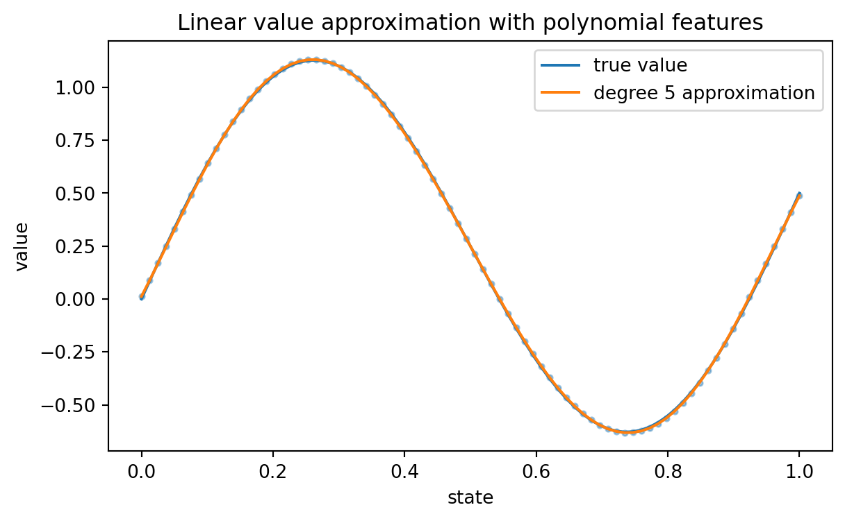
The following example creates a smooth value function over a one-dimensional state space and approximates it with polynomial features. This is ordinary weighted least squares, but the interpretation is RL-specific: the target is a value function and the weights represent a state-visitation distribution.
import numpy as npimport matplotlib.pyplot as pltstates = np.linspace(0, 1, 80)true_V = np.sin(2* np.pi * states) +0.5* states# A state weighting: later states are visited more often.d =0.5+ statesd = d / d.sum()D = np.diag(d)def polynomial_features(x, degree):return np.column_stack([x**k for k inrange(degree +1)])for degree in [1, 3, 7]: Phi = polynomial_features(states, degree) theta = np.linalg.solve(Phi.T @ D @ Phi, Phi.T @ D @ true_V) fitted = Phi @ theta weighted_mse = np.sum(d * (true_V - fitted)**2)print(f"degree={degree:2d}, weighted MSE={weighted_mse:.5f}")Phi = polynomial_features(states, 5)theta = np.linalg.solve(Phi.T @ D @ Phi, Phi.T @ D @ true_V)fitted = Phi @ thetaplt.figure(figsize=(7, 4))plt.plot(states, true_V, label="true value")plt.plot(states, fitted, label="degree 5 approximation")plt.scatter(states, fitted, s=8, alpha=0.4)plt.xlabel("state")plt.ylabel("value")plt.title("Linear value approximation with polynomial features")plt.legend()plt.show()
Polynomial feature approximation of a value function.
This example is supervised regression only because the true \(V\) is supplied. In reinforcement learning, \(V^\pi\) is usually unknown. We observe sampled rewards and transitions, and the target itself depends on the current approximation.
16.6 13.5 Bellman backups leave the feature space
For a fixed policy \(\pi\), the Bellman expectation operator is
\[
T^\pi V = r_\pi + \gamma P_\pi V.
\]
If \(V\) belongs to the feature space \(\mathcal L=\operatorname{col}(\Phi)\), then \(T^\pi V\) need not belong to \(\mathcal L\). That is,
\[
V \in \mathcal L
\quad \not\Rightarrow \quad
T^\pi V \in \mathcal L.
\]
This is the fundamental reason projection enters approximate dynamic programming. We cannot usually solve
\[
V = T^\pi V
\]
inside the feature space. Instead, we solve the projected Bellman equation
\[
\Phi^T D(I-\gamma P_\pi)\Phi\theta
=\Phi^T D r_\pi.
\]
Define
\[
A=\Phi^T D(I-\gamma P_\pi)\Phi,
\qquad
b=\Phi^T D r_\pi.
\]
Then the projected Bellman equation becomes the linear system
\[
A\theta=b.
\]
When \(A\) is nonsingular, the solution is
\[
\theta_{\mathrm{PBE}}=A^{-1}b.
\]
16.6.1 Interactive: Bellman backup followed by projection
The Bellman operator moves the current approximate value function toward dynamic consistency. Projection moves it back into the chosen feature space. The projected Bellman fixed point is where these two operations balance.
Notice that the projected Bellman solution and the projection of the exact value are not generally the same. The projected Bellman solution solves a dynamic consistency equation after projection; the least-squares projection solves a pure approximation problem.
16.8 13.7 Three different errors
Approximate value prediction involves several losses. They are related but not identical.
This measures Bellman inconsistency. It is natural but difficult to estimate from single samples because the squared conditional expectation is not the expectation of a squared single-sample target.
The projected Bellman equation is equivalent to minimizing the MSPBE to zero when an exact projected fixed point exists.
Do not confuse these objectives. Least-squares regression targets MSVE. Bellman residual methods target MSBE. TD methods with linear approximation are connected to the projected Bellman equation and MSPBE.
16.9 13.8 Semi-gradient TD with linear approximation
For a differentiable value approximation \(V_\theta(s)\), the TD error is
This update is widely used, but it is also a warning sign: the combination of bootstrapping, off-policy sampling, and function approximation can be unstable.
16.12 13.11 The deadly triad
Approximate RL is not merely tabular RL with fewer parameters. Stability can change dramatically. A classical warning is the deadly triad:
function approximation, which generalizes across states;
bootstrapping, which uses current value estimates inside the target;
off-policy learning, where the data distribution differs from the target policy.
When all three are present, divergence can occur even in small linear examples. This is one reason modern deep RL uses stabilization devices such as replay buffers, target networks, trust-region updates, and conservative objectives.
For fixed-policy on-policy prediction with linear features, TD has strong convergence theory under suitable conditions. For nonlinear, off-policy, or control settings, the analysis is more delicate.
16.13 13.12 Bias, variance, and feature complexity
Feature choice controls an approximation tradeoff. With too few features, the model cannot represent the true value function well. With too many features, the estimate can become noisy or ill-conditioned.
Let \(\mathcal F_d\) be a sequence of approximation spaces of increasing dimension. The expected prediction error often follows the qualitative decomposition
\[
\mathbb E\lVert V^\pi-\widehat V_d\rVert_D^2
\approx
\underbrace{\text{bias}(d)^2}_{\text{decreases with complexity}}
+
\underbrace{\text{variance}(d)}_{\text{increases with complexity}}
+
\underbrace{\text{irreducible noise}}_{\text{sampling uncertainty}}.
\]
This is familiar from statistical learning, but RL adds complications: the data are dependent, the target is bootstrapped, and the state distribution depends on the policy.
16.13.1 Interactive: Feature complexity and prediction error
As the number of features increases, approximation error decreases at first. But with limited noisy data, high-complexity models can become unstable or overfit the sampled returns.
16.14 13.13 Neural value functions
A neural value function replaces linear features by learned nonlinear features. A neural network value function can be written abstractly as
\[
V_\theta(s)=f_\theta(s),
\]
where \(\theta\) includes all weights and biases. A neural action-value function has the form
\[
Q_\theta(s,a)=f_\theta(s,a)
\]
or, for discrete actions, a network may output a vector
\[
(Q_\theta(s,a_1),\ldots,Q_\theta(s,a_m)).
\]
The TD loss used in many deep RL algorithms has the form
The parameter vector \(\theta^-\) is a delayed target-network parameter. This separates the rapidly changing prediction network from the target used in the update.
The mathematical picture remains the same:
\[
\text{choose a function class, define a Bellman-style target, and optimize a sample-based objective.}
\]
The analysis becomes harder because the objective is nonconvex and the target distribution changes during learning.
16.15 13.14 AI-assisted component: choosing features responsibly
Large language models can help generate feature ideas, but they can also produce features that leak future information, violate the Markov property, or encode irrelevant proxies. For mathematical RL work, an AI assistant should be used as a critic rather than as an authority.
AI prompt: feature audit
Consider an RL problem with state variables, actions, rewards, and a proposed feature map \(\phi(s)\) or \(\phi(s,a)\). Ask an AI assistant:
Which features are functions only of information available at decision time?
Which features might leak future rewards or next states?
Which features help preserve the Markov property?
Which features create near-collinearity or poor conditioning?
Which omitted variables could cause systematic value approximation bias?
Then translate the answer into a mathematical checklist involving \(\Phi^TD\Phi\), state coverage, policy dependence, and the target value function.
AI prompt: debugging approximate TD code
Paste a TD update and ask the assistant to identify:
the sampled state \(S_t\) and next state \(S_{t+1}\);
the TD target;
the TD error;
whether the update is a full gradient or semi-gradient;
whether the method is on-policy or off-policy;
whether terminal states are handled correctly.
Do not accept the answer until every item is matched to a line of code.
16.16 13.15 Summary
Function approximation is the mathematical step that allows reinforcement learning to scale beyond tables. The main ideas are:
a value function is approximated by a parameterized family \(V_\theta\);
linear approximation uses \(V_\theta=\Phi\theta\);
weighted least squares projects values using the state distribution \(D\);
Bellman backups generally leave the feature space;
projected Bellman equations combine dynamic consistency with approximation;
semi-gradient TD learns the projected Bellman solution from samples in the linear on-policy prediction setting;
approximate control is powerful but can be unstable;
feature complexity creates a bias-variance tradeoff;
neural value functions extend the same ideas to learned nonlinear representations.
The next chapter studies stochastic approximation more systematically. That theory explains why update rules such as TD can converge despite noisy samples.
16.17 Exercises
16.17.1 Conceptual exercises
Explain why tabular value functions do not generalize across states.
In \(V_\theta(s)=\phi(s)^T\theta\), what is linear and what may be nonlinear?
Why should approximation error be measured using a state distribution \(d(s)\)?
Explain the difference between projecting \(V^\pi\) and solving the projected Bellman equation.
Why is semi-gradient TD not the same as ordinary supervised gradient descent?
State the deadly triad and explain why each component matters.
16.17.2 Mathematical exercises
Let \(D\) be a positive diagonal matrix and \(\Phi\) have full column rank. Prove that
\[
\Pi_D=\Phi(\Phi^TD\Phi)^{-1}\Phi^TD
\]
satisfies \(\Pi_D^2=\Pi_D\).
Prove that the residual \(V-\Pi_DV\) is \(D\)-orthogonal to \(\operatorname{col}(\Phi)\).
Starting from
\[
\Phi\theta = \Pi_D(r+\gamma P\Phi\theta),
\]
derive the linear system
\[
\Phi^TD(I-\gamma P)\Phi\theta=\Phi^TD r.
\]
For a two-state Markov reward process, choose one constant feature \(\phi(s)=1\). Derive the projected Bellman equation explicitly.
Show that if \(\operatorname{col}(\Phi)=\mathbb R^n\), then the projected Bellman equation reduces to the exact Bellman equation.
16.17.3 Computational exercises
Modify the polynomial approximation example using Fourier features instead of polynomial features.
Estimate the state distribution \(d\) from a simulated trajectory and recompute the least-squares projection.
Compare the projected Bellman solution with the least-squares projection of the exact value for several feature matrices.
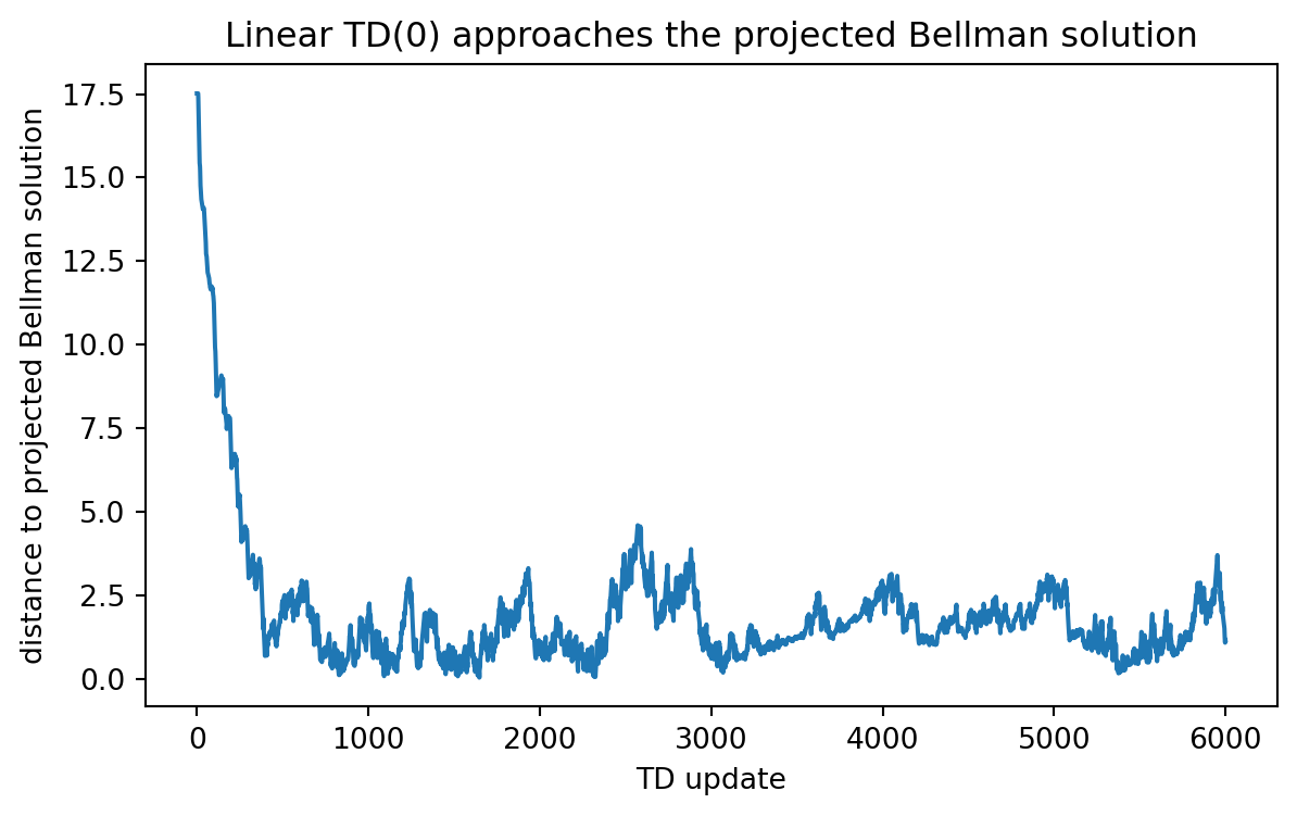
Implement linear TD(0) with three different learning rates and compare convergence behavior.
Implement approximate SARSA using a feature vector \(\phi(s,a)\) for a small gridworld.
Test how the condition number of \(\Phi^TD\Phi\) changes as more polynomial features are added.
16.17.4 AI-assisted exercises
Ask an AI assistant to propose features for an inventory-control problem. Identify which features are mathematically valid state variables.
Ask an AI assistant to explain the difference between MSVE, MSBE, and MSPBE. Correct any imprecise statements.
Give an AI assistant a TD update and ask whether it is on-policy or off-policy. Verify its answer algebraically.
Ask an AI assistant to rewrite the projected Bellman equation in matrix form, then check every dimension.
Ask an AI assistant to suggest diagnostics for instability in approximate Q-learning. Translate each diagnostic into a mathematical quantity or plot.
16.18 Instructor notes
This chapter is a bridge between tabular dynamic programming and modern deep reinforcement learning. For MA Applied Math and MS Statistics students, emphasize three connections:
Linear algebra: feature spaces, projections, normal equations, conditioning.
Probability: state distributions, sampled transitions, dependent data.
Optimization: semi-gradient updates, stochastic approximation, and objective mismatch.
A useful lecture sequence is: start with least-squares projection, then show that Bellman backups leave the feature space, then derive the projected Bellman equation, then derive linear TD as a stochastic approximation to that equation.