19  Actor-Critic Methods

Core idea. Actor-critic methods combine two approximations. The actor is a parameterized policy \(\pi_\theta(a\mid s)\) that chooses actions. The critic is a value-function approximation, such as \(V_w(s)\) or \(Q_w(s,a)\), that evaluates the actor. The critic supplies a low-variance estimate of the advantage of the sampled action, and the actor uses that estimate to update the policy.

A common one-step actor-critic update is

\[ \delta_t = R_{t+1}+\gamma V_w(S_{t+1})-V_w(S_t), \]

\[ w_{t+1}=w_t+\beta_t\delta_t\nabla_w V_w(S_t), \]

\[ \theta_{t+1} = \theta_t + \alpha_t\delta_t\nabla_\theta\log \pi_\theta(A_t\mid S_t). \]

The update should be read as policy-gradient learning with a learned baseline and a learned advantage estimator.

19.1 Learning goals

After reading this chapter, students should be able to:

1. describe the actor, critic, value baseline, advantage estimate, and TD error;
2. derive the one-step actor-critic update from the policy gradient theorem;
3. explain why the TD error can be interpreted as a sample advantage;
4. distinguish Monte Carlo policy gradient, TD actor-critic, \(n\)-step actor-critic, and advantage actor-critic;
5. implement a tabular actor-critic algorithm for a small episodic MDP;
6. explain the role of two-time-scale stochastic approximation;
7. define generalized advantage estimation and explain the bias-variance role of \(\lambda\);
8. identify instability sources in actor-critic learning;
9. use AI tools to audit derivations, implementation details, and modeling assumptions.

19.2 16.1 Why actor-critic methods?

Policy gradient methods from Chapter 15 estimate

\[ \nabla_\theta J(\theta) = \mathbb E_{\pi_\theta} \left[ \nabla_\theta\log\pi_\theta(A_t\mid S_t) Q^{\pi_\theta}(S_t,A_t) \right]. \]

The REINFORCE algorithm replaces \(Q^{\pi_\theta}(S_t,A_t)\) by an observed return \(G_t\). This gives an unbiased estimator in many episodic settings, but the estimator may have high variance because a full trajectory return includes many random rewards unrelated to the sampled action.

Actor-critic methods reduce this variance by learning a critic. Instead of using the full return \(G_t\), the actor uses a value-based estimate of how much better the sampled action was than the policy’s typical behavior in that state. This estimate is often based on the temporal-difference error.

The main idea is

\[ \text{policy gradient} + \text{learned value baseline} + \text{bootstrapping} = \text{actor-critic}. \]

For MA Applied Math students, actor-critic is a coupled stochastic approximation method. For MS Statistics students, actor-critic is a sequential estimation method in which a nuisance function, the value function, is learned to reduce the variance of a policy-gradient estimator.

The critic does not replace the actor. It supplies information about the actor’s current policy. The actor changes the policy; the critic evaluates the policy being changed.

19.2.1 Interactive: Actor-critic information flow

The actor generates actions, the environment generates rewards and next states, and the critic turns the transition into a TD error. That scalar TD error updates both the critic and the actor.

19.3 16.2 The advantage function

For a fixed policy \(\pi\), the state-value and action-value functions are

\[ V^\pi(s) = \mathbb E_\pi \left[ \sum_{k=0}^{\infty}\gamma^kR_{t+k+1} \mid S_t=s \right], \]

and

\[ Q^\pi(s,a) = \mathbb E_\pi \left[ \sum_{k=0}^{\infty}\gamma^kR_{t+k+1} \mid S_t=s,A_t=a \right]. \]

The advantage function is

\[ A^\pi(s,a)=Q^\pi(s,a)-V^\pi(s). \]

It measures whether action \(a\) is better or worse than the policy’s average action choice at state \(s\). Since

\[ V^\pi(s)=\sum_a\pi(a\mid s)Q^\pi(s,a), \]

we have

\[ \sum_a\pi(a\mid s)A^\pi(s,a)=0. \]

Thus the advantage is centered under the current policy.

The policy gradient theorem can be written using the advantage:

\[ \nabla_\theta J(\theta) = \mathbb E_{\pi_\theta} \left[ \nabla_\theta\log\pi_\theta(A_t\mid S_t) A^{\pi_\theta}(S_t,A_t) \right]. \]

This is valid because subtracting any state-dependent baseline \(b(s)\) does not change the expectation:

\[ \mathbb E_{A\sim\pi_\theta(\cdot\mid s)} \left[ \nabla_\theta\log\pi_\theta(A\mid s)b(s) \right] = b(s)\nabla_\theta\sum_a\pi_\theta(a\mid s) = 0. \]

The special baseline \(b(s)=V^{\pi_\theta}(s)\) turns \(Q^{\pi_\theta}\) into \(A^{\pi_\theta}\).

19.4 16.3 TD error as a sample advantage

Suppose the critic were exact, so that \(V_w=V^\pi\). Define the one-step TD error

\[ \delta_t = R_{t+1}+\gamma V^\pi(S_{t+1})-V^\pi(S_t). \]

Conditioning on \(S_t=s\) and \(A_t=a\), we obtain

\[ \mathbb E_\pi[\delta_t\mid S_t=s,A_t=a] = \mathbb E_\pi \left[ R_{t+1}+\gamma V^\pi(S_{t+1}) \mid S_t=s,A_t=a \right] - V^\pi(s). \]

The first conditional expectation is \(Q^\pi(s,a)\). Therefore

\[ \mathbb E_\pi[\delta_t\mid S_t=s,A_t=a] = Q^\pi(s,a)-V^\pi(s) = A^\pi(s,a). \]

This identity explains the central actor-critic update. The TD error is a noisy one-step sample of the advantage.

19.4.1 Interactive: TD error as a sample advantage

The TD error is random because reward and next state are random. Its conditional mean is the advantage when the critic is correct.

19.5 16.4 The actor and the critic

An actor-critic algorithm maintains two parameter vectors:

\[ \theta\in\mathbb R^d \quad\text{and}\quad w\in\mathbb R^m. \]

The actor is a differentiable policy

\[ \pi_\theta(a\mid s), \]

and the critic is usually one of the following:

\[ V_w(s), \qquad Q_w(s,a), \qquad A_w(s,a). \]

The most common introductory version uses a state-value critic \(V_w(s)\). Given a transition

\[ (S_t,A_t,R_{t+1},S_{t+1}), \]

we compute

\[ \delta_t = R_{t+1}+\gamma V_w(S_{t+1})-V_w(S_t). \]

For a differentiable critic, a semi-gradient TD update is

\[ w_{t+1} = w_t+\beta_t\delta_t\nabla_w V_w(S_t). \]

The actor update is

\[ \theta_{t+1} = \theta_t+ \alpha_t\delta_t\nabla_\theta\log\pi_\theta(A_t\mid S_t). \]

The critic update moves \(V_w(S_t)\) toward the bootstrapped target

\[ R_{t+1}+\gamma V_w(S_{t+1}), \]

whereas the actor update increases the log-probability of \(A_t\) if \(\delta_t>0\) and decreases it if \(\delta_t<0\).

19.6 16.5 Tabular softmax actor

For a finite state-action problem, a convenient actor is a tabular softmax policy. Let \(h_\theta(s,a)\) be a preference parameter. Define

\[ \pi_\theta(a\mid s) = \frac{\exp(h_\theta(s,a))} {\sum_b\exp(h_\theta(s,b))}. \]

For the parameter \(h_\theta(s,b)\), the score is

\[ \frac{\partial}{\partial h_\theta(s,b)} \log\pi_\theta(a\mid s) = \mathbf 1\{a=b\}-\pi_\theta(b\mid s). \]

Therefore, in the visited state \(s=S_t\), the actor update for each action \(b\) is

\[ h(s,b) \leftarrow h(s,b)+ \alpha_t\delta_t \left(\mathbf 1\{A_t=b\}-\pi(b\mid s)\right). \]

This update increases the relative preference of the selected action if the TD error is positive and decreases it if the TD error is negative.

19.7 16.6 Tabular state-value critic

For a tabular critic, let \(V_w(s)=w_s\). Then

\[ \nabla_w V_w(S_t)=e_{S_t}, \]

where \(e_{S_t}\) is a coordinate vector. The critic update becomes

\[ V(S_t) \leftarrow V(S_t)+\beta_t \left[ R_{t+1}+\gamma V(S_{t+1})-V(S_t) \right]. \]

This is exactly the TD(0) policy-evaluation update, except the policy being evaluated is changing over time.

Tabular one-step actor-critic

Initialize policy preferences \(h(s,a)\) and values \(V(s)\).

For each episode:

1. Start from an initial state \(S_0\).
2. At time \(t\), sample \(A_t\sim\pi_h(\cdot\mid S_t)\).
3. Observe \(R_{t+1}\) and \(S_{t+1}\).
4. Compute \(\delta_t=R_{t+1}+\gamma V(S_{t+1})-V(S_t)\).
5. Update \(V(S_t)\leftarrow V(S_t)+\beta_t\delta_t\).
6. For each action \(b\), update

\[ h(S_t,b) \leftarrow h(S_t,b)+\alpha_t\delta_t \left(\mathbf 1\{A_t=b\}-\pi_h(b\mid S_t)\right). \]

7. Continue until termination.

19.8 16.7 Python example: exact advantages in a tiny MDP

We begin with a two-state episodic MDP. State \(2\) is terminal. In state \(0\), action \(1\) moves toward state \(1\), while action \(0\) tends to keep the process in state \(0\). In state \(1\), action \(1\) tends to reach the terminal reward.

import numpy as np

np.set_printoptions(precision=4, suppress=True)

gamma = 0.95
n_states = 3
n_actions = 2
terminal = 2

# P[s, a, s_next]
P = np.zeros((n_states, n_actions, n_states))
R = np.zeros((n_states, n_actions, n_states))

# State 0
P[0, 0, 0] = 0.85
P[0, 0, 1] = 0.15
P[0, 1, 0] = 0.25
P[0, 1, 1] = 0.75

# State 1
P[1, 0, 0] = 0.70
P[1, 0, 1] = 0.30
P[1, 1, 1] = 0.20
P[1, 1, 2] = 0.80
R[1, 1, 2] = 1.0

# Terminal state
P[2, :, 2] = 1.0

# A fixed stochastic policy
pi = np.array([
    [0.55, 0.45],
    [0.35, 0.65],
    [0.50, 0.50]
])

P_pi = np.einsum("sa,san->sn", pi, P)
r_sa = np.einsum("san,san->sa", P, R)
r_pi = np.sum(pi * r_sa, axis=1)

A_mat = np.eye(n_states) - gamma * P_pi
V = np.linalg.solve(A_mat, r_pi)

Q = r_sa + gamma * np.einsum("san,n->sa", P, V)
Adv = Q - V[:, None]

print("V^pi:")
print(V)
print("\nQ^pi:")
print(Q)
print("\nA^pi:")
print(Adv)
print("\nPolicy-weighted advantage by state:")
print(np.sum(pi * Adv, axis=1))

V^pi:
[0.8108 0.9124 0.    ]

Q^pi:
[[0.7847 0.8427]
 [0.7992 0.9734]
 [0.     0.    ]]

A^pi:
[[-0.0261  0.0319]
 [-0.1132  0.0609]
 [ 0.      0.    ]]

Policy-weighted advantage by state:
[-0.  0.  0.]

The last line should be close to zero. This verifies the centering identity

\[ \sum_a\pi(a\mid s)A^\pi(s,a)=0. \]

19.9 16.8 Python example: tabular actor-critic

The next example implements a small actor-critic algorithm from scratch.

import numpy as np
import matplotlib.pyplot as plt

rng = np.random.default_rng(7243)

def softmax(x):
    z = x - np.max(x)
    e = np.exp(z)
    return e / e.sum()

def step(state, action, rng):
    probs = P[state, action]
    next_state = rng.choice(n_states, p=probs)
    reward = R[state, action, next_state]
    done = next_state == terminal
    return next_state, reward, done

h = np.zeros((n_states, n_actions))
V_est = np.zeros(n_states)
alpha = 0.06
beta = 0.15
num_episodes = 2000
returns = []
prob_good_0 = []
prob_good_1 = []

for episode in range(num_episodes):
    state = 0
    total_reward = 0.0
    discount = 1.0
    for t in range(100):
        probs = softmax(h[state])
        action = rng.choice(n_actions, p=probs)
        next_state, reward, done = step(state, action, rng)
        td_target = reward + gamma * V_est[next_state] * (not done)
        delta = td_target - V_est[state]

        # Critic update
        V_est[state] += beta * delta

        # Actor update for tabular softmax preferences
        grad_log = -probs
        grad_log[action] += 1.0
        h[state] += alpha * delta * grad_log

        total_reward += discount * reward
        discount *= gamma
        state = next_state
        if done:
            break

    returns.append(total_reward)
    prob_good_0.append(softmax(h[0])[1])
    prob_good_1.append(softmax(h[1])[1])

window = 50
smoothed = np.convolve(returns, np.ones(window) / window, mode="valid")

plt.figure(figsize=(7, 4))
plt.plot(smoothed)
plt.xlabel("episode")
plt.ylabel("moving average discounted return")
plt.title("Tabular actor-critic learning curve")
plt.show()

print("Estimated values:", V_est)
print("Policy at state 0:", softmax(h[0]))
print("Policy at state 1:", softmax(h[1]))

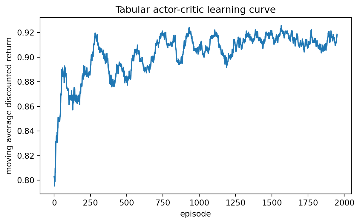
A tabular actor-critic algorithm learns to move from state 0 to state 1 and then to the terminal reward.

Estimated values: [0.9237 0.9879 0.    ]
Policy at state 0: [0.0711 0.9289]
Policy at state 1: [0.031 0.969]

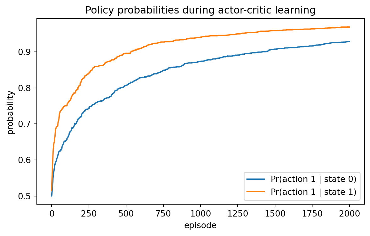
The policy should learn to prefer action \(1\) in both nonterminal states. In state \(0\), action \(1\) moves the agent toward state \(1\). In state \(1\), action \(1\) moves the agent toward the terminal reward.

plt.figure(figsize=(7, 4))
plt.plot(prob_good_0, label="Pr(action 1 | state 0)")
plt.plot(prob_good_1, label="Pr(action 1 | state 1)")
plt.xlabel("episode")
plt.ylabel("probability")
plt.title("Policy probabilities during actor-critic learning")
plt.legend()
plt.show()

The actor gradually increases the probability of useful actions.

19.10 16.9 Actor-critic as coupled stochastic approximation

The actor and critic are updated from the same trajectory, so actor-critic algorithms are coupled stochastic approximation schemes. A useful abstract form is

\[ w_{t+1} = w_t+\beta_t \left[g(w_t,\theta_t)+M_{t+1}^{(w)}\right], \]

\[ \theta_{t+1} = \theta_t+ \alpha_t \left[f(w_t,\theta_t)+M_{t+1}^{(\theta)}\right]. \]

Here \(M_{t+1}^{(w)}\) and \(M_{t+1}^{(\theta)}\) are noise terms. Often the critic is trained on a faster time scale than the actor:

\[ \frac{\alpha_t}{\beta_t}\to 0. \]

Intuitively, the critic nearly equilibrates for the current actor before the actor changes substantially. This separation is mathematically useful because the actor can then be analyzed as if it were receiving approximately correct value estimates.

19.10.1 Interactive: Two-time-scale learning

The critic usually needs to track the current policy faster than the actor changes it. When the actor moves too quickly, the critic may evaluate a policy that is already outdated.

19.11 16.10 \(n\)-step actor-critic

The one-step TD error uses a short bootstrap target. More generally, an \(n\)-step target is

\[ G_t^{(n)} = R_{t+1}+\gamma R_{t+2}+\cdots+ \gamma^{n-1}R_{t+n} + \gamma^n V_w(S_{t+n}). \]

The corresponding advantage estimate is

\[ \widehat A_t^{(n)}=G_t^{(n)}-V_w(S_t). \]

The actor update becomes

\[ \theta_{t+1} = \theta_t+ \alpha_t \widehat A_t^{(n)} \nabla_\theta\log\pi_\theta(A_t\mid S_t). \]

Small \(n\) gives more bootstrapping and often lower variance. Large \(n\) uses more observed rewards and often lower bias when the critic is inaccurate.

19.12 16.11 Advantage actor-critic and batch updates

In modern implementations, one often collects a batch of transitions or short rollouts before updating the parameters. Suppose a batch contains samples indexed by \(i\). Let \(\widehat A_i\) be an advantage estimate. The actor objective is often written as

\[ L_{\text{actor}}(\theta) = -\frac{1}{N} \sum_{i=1}^N \log\pi_\theta(a_i\mid s_i)\widehat A_i. \]

Minimizing this loss by gradient descent is equivalent to policy-gradient ascent. The critic loss is commonly

\[ L_{\text{critic}}(w) = \frac{1}{2N}\sum_{i=1}^N \left(\widehat G_i-V_w(s_i)\right)^2. \]

A typical combined loss is

\[ L(\theta,w) = L_{\text{actor}}(\theta) +c_vL_{\text{critic}}(w) -c_H\frac{1}{N}\sum_{i=1}^NH(\pi_\theta(\cdot\mid s_i)), \]

where \(H\) is policy entropy. The entropy term encourages exploration.

19.12.1 Interactive: Batch advantage actor-critic update

A batch update averages several noisy advantage estimates before changing the actor. Larger batches reduce gradient noise but require more data before each update.

19.13 16.12 Generalized advantage estimation

Generalized advantage estimation, or GAE, combines TD errors across multiple horizons. Define the one-step TD residual

\[ \delta_t = R_{t+1}+\gamma V_w(S_{t+1})-V_w(S_t). \]

The GAE estimator is

\[ \widehat A_t^{\text{GAE}(\gamma,\lambda)} = \sum_{l=0}^{\infty}(\gamma\lambda)^l\delta_{t+l}. \]

The parameter \(\lambda\in[0,1]\) controls a bias-variance tradeoff:

• \(\lambda=0\) gives the one-step TD advantage \(\delta_t\);
• larger \(\lambda\) includes longer sequences of TD residuals;
• \(\lambda\) close to \(1\) approaches a Monte Carlo-like advantage estimate.

19.13.1 Interactive: GAE weights

GAE uses geometrically decaying weights \((\gamma\lambda)^l\) on future TD residuals. Larger \(\lambda\) spreads credit over more future residuals.

19.14 16.13 Entropy regularization

Actor-critic methods may prematurely collapse to nearly deterministic policies. Entropy regularization discourages this collapse by adding

\[ H(\pi_\theta(\cdot\mid s)) = -\sum_a\pi_\theta(a\mid s) \log\pi_\theta(a\mid s) \]

to the objective. A regularized objective has the schematic form

\[ J_H(\theta) = \mathbb E_{\pi_\theta} \left[ \sum_{t=0}^{\infty}\gamma^t \left(R_{t+1}+\eta H(\pi_\theta(\cdot\mid S_t))\right) \right]. \]

The coefficient \(\eta>0\) controls how strongly the method values exploration. Too little entropy may cause early policy collapse. Too much entropy may prevent the policy from exploiting learned structure.

19.14.1 Interactive: Entropy-regularized actor update

Entropy regularization keeps action probabilities away from zero while the advantage term pushes probability toward useful actions.

19.15 16.14 Python example: GAE from a sequence of TD errors

The following function computes GAE for a finite rollout.

import numpy as np

def generalized_advantage_estimate(rewards, values, gamma=0.99, lam=0.95):
    """Compute GAE for one finite rollout.

    rewards has length T.
    values has length T + 1 and includes the bootstrap value.
    """
    T = len(rewards)
    advantages = np.zeros(T)
    gae = 0.0
    for t in reversed(range(T)):
        delta = rewards[t] + gamma * values[t + 1] - values[t]
        gae = delta + gamma * lam * gae
        advantages[t] = gae
    return advantages

rewards = np.array([0.0, 0.0, 1.0, 0.0, 2.0])
values = np.array([0.30, 0.35, 0.60, 0.40, 1.10, 0.00])

for lam in [0.0, 0.5, 0.95, 1.0]:
    adv = generalized_advantage_estimate(rewards, values, gamma=0.9, lam=lam)
    print(f"lambda={lam:0.2f}: {adv}")

lambda=0.00: [0.015 0.19  0.76  0.59  0.9  ]
lambda=0.50: [0.3451 0.7335 1.2078 0.995  0.9   ]
lambda=0.95: [1.5828 1.8336 1.9224 1.3595 0.9   ]
lambda=1.00: [1.8222 2.008  2.02   1.4    0.9   ]

This code makes the role of \(\lambda\) concrete: larger \(\lambda\) lets later TD residuals influence earlier updates more strongly.

19.16 16.15 Actor-critic with function approximation

For large state spaces, both actor and critic are usually approximated. A common linear critic is

\[ V_w(s)=\phi(s)^Tw, \]

where \(\phi(s)\) is a feature vector. The critic update is

\[ w_{t+1} = w_t+\beta_t\delta_t\phi(S_t). \]

For a softmax actor with features \(\psi(s,a)\),

\[ \pi_\theta(a\mid s) = \frac{\exp(\theta^T\psi(s,a))} {\sum_b\exp(\theta^T\psi(s,b))}, \]

and

\[ \nabla_\theta\log\pi_\theta(a\mid s) = \psi(s,a)-\sum_b\pi_\theta(b\mid s)\psi(s,b). \]

The actor update is

\[ \theta_{t+1} = \theta_t+ \alpha_t\delta_t \left(\psi(S_t,A_t)-\sum_b\pi_\theta(b\mid S_t)\psi(S_t,b)\right). \]

With nonlinear function approximation, such as neural networks, the same equations are implemented by automatic differentiation. The mathematical meaning remains the same: the critic estimates a value baseline, and the actor increases the probability of actions with positive estimated advantage.

19.17 16.16 Stability issues

Actor-critic methods are powerful but delicate. Common sources of instability include:

• the critic is inaccurate and gives misleading advantage estimates;
• the actor changes too quickly for the critic to track;
• the policy becomes nearly deterministic too early;
• off-policy data are used without correction;
• bootstrapping and function approximation amplify errors;
• advantage estimates have high variance;
• learning rates are poorly scaled.

Useful diagnostics include:

• average episodic return;
• critic loss or TD-error magnitude;
• policy entropy;
• gradient norms;
• approximate KL divergence between old and new policies;
• distribution of estimated advantages;
• fraction of actions with near-zero probability.

Actor-critic should not be interpreted as a guaranteed gradient method unless the critic, sampling distribution, and update schedule satisfy additional assumptions. In practice, actor-critic is a family of approximate stochastic optimization methods.

19.18 16.17 AI-assisted learning components

19.18.1 AI prompt: deriving the actor update

Ask an AI assistant:

Starting from the policy gradient theorem, derive the one-step actor-critic update using the TD error as an advantage estimate. Explicitly state where an approximation is introduced.

A good answer should identify the exact identity

\[ \nabla_\theta J(\theta) = \mathbb E \left[ \nabla_\theta\log\pi_\theta(A_t\mid S_t)A^{\pi_\theta}(S_t,A_t) \right] \]

and then explain that \(A^{\pi_\theta}\) is replaced by the sample TD error computed from an approximate critic.

19.18.2 AI prompt: debugging actor-critic code

Ask an AI assistant to check the following implementation points:

1. Are terminal states handled correctly in the TD target?
2. Is the actor using \(\nabla_\theta\log\pi_\theta(A_t\mid S_t)\) rather than \(\nabla_\theta\pi_\theta(A_t\mid S_t)\)?
3. Is the advantage estimate detached from the actor computation when using neural-network libraries?
4. Are actor and critic learning rates separated?
5. Is entropy being maximized rather than minimized?

19.18.3 AI prompt: experiment critique

Give an AI assistant a plot of returns, value losses, entropy, and gradient norms. Ask it to propose three possible failure modes and three follow-up experiments. The answer should distinguish evidence from speculation.

19.19 16.18 Summary

Actor-critic methods combine policy-gradient optimization with value-function estimation. The actor changes the policy, while the critic estimates the quality of the current policy. The central bridge between them is the TD error:

\[ \delta_t=R_{t+1}+\gamma V_w(S_{t+1})-V_w(S_t). \]

When the critic is accurate, the conditional expectation of \(\delta_t\) is the advantage \(A^\pi(s,a)\). This makes the TD error a natural low-variance substitute for a Monte Carlo return in the policy-gradient update.

The main mathematical themes are:

• score-function gradients;
• baselines and advantage functions;
• Bellman equations;
• temporal-difference learning;
• stochastic approximation;
• two-time-scale dynamics;
• bias-variance tradeoffs in advantage estimation.

19.20 Exercises

19.20.1 Conceptual exercises

1. Explain the difference between an actor and a critic.
2. Why is \(V^\pi(s)\) a natural baseline for policy gradients?
3. Explain why the TD error is not exactly the advantage when the critic is approximate.
4. Why can a critic reduce variance but introduce bias?
5. Explain why entropy regularization can help exploration.

19.20.2 Mathematical exercises

1. Prove that for any function \(b(s)\),

\[ \mathbb E_{A\sim\pi_\theta(\cdot\mid s)} \left[ \nabla_\theta\log\pi_\theta(A\mid s)b(s) \right]=0. \]

2. Suppose \(V_w=V^\pi\). Prove that

\[ \mathbb E[\delta_t\mid S_t=s,A_t=a]=A^\pi(s,a). \]

3. Derive the softmax score formula

\[ \frac{\partial}{\partial h(s,b)}\log\pi(a\mid s) = \mathbf 1\{a=b\}-\pi(b\mid s). \]

4. Show that GAE with \(\lambda=0\) equals the one-step TD residual.

5. For a finite rollout, write \(\widehat A_t^{\text{GAE}}\) recursively as

\[ \widehat A_t=\delta_t+\gamma\lambda\widehat A_{t+1}. \]

19.20.3 Computational exercises

1. Modify the tabular actor-critic example by changing \(\alpha\) and \(\beta\). What happens when \(\alpha\) is much larger than \(\beta\)?
2. Add entropy regularization to the tabular actor update.
3. Replace the one-step TD error by a three-step advantage estimate.
4. Plot the distribution of TD errors during learning.
5. Compare actor-critic with REINFORCE on the same tiny MDP.

19.20.4 AI-assisted exercises

1. Ask an AI assistant to derive the actor-critic update. Then identify one step in the derivation that relies on approximation.
2. Ask an AI assistant to inspect actor-critic code and identify terminal-state bugs.
3. Ask an AI assistant to design diagnostics for unstable actor-critic training.
4. Ask an AI assistant to explain the difference between A2C, A3C, and PPO in mathematical terms.
5. Ask an AI assistant to critique whether a proposed reward function is likely to produce unintended behavior.

19.21 Notes for instructors

This chapter is a natural synthesis point. Students have already seen policy gradients, TD learning, and stochastic approximation. The lecture can be organized around one identity:

\[ \mathbb E[\delta_t\mid S_t=s,A_t=a]=A^\pi(s,a) \]

when the critic is exact. This identity makes actor-critic methods feel inevitable rather than mysterious.

For MA Applied Math students, emphasize coupled stochastic approximation, fixed points, and two-time-scale dynamics. For MS Statistics students, emphasize baselines, variance reduction, conditional expectations, nuisance estimation, and diagnostics.