21 Policy Optimization

Core idea. Policy optimization methods update a parameterized policy directly. Instead of first learning a table of optimal action values and then acting greedily, we choose a differentiable family of policies \(\{\pi_\theta:\theta\in\Theta\}\) and try to solve

\[ \max_{\theta\in\Theta} J(\theta), \]

where \(J(\theta)\) is the expected long-run return under \(\pi_\theta\). The mathematical difficulty is that a small change in \(\theta\) can change both the action probabilities and the distribution of future states. Modern methods such as TRPO and PPO stabilize policy-gradient learning by controlling how far the new policy moves from the old policy.

21.1 Learning goals

After reading this chapter, students should be able to:

define the policy objective \(J(\theta)\) for discounted episodic and continuing problems;
derive the likelihood-ratio form of the policy-gradient update;
state the performance difference lemma and interpret it statistically;
explain why policy optimization uses data collected from an old policy;
derive the probability ratio \(r_t(\theta)\) used in PPO;
explain KL divergence as a local geometry on the space of policies;
distinguish vanilla policy gradient, natural policy gradient, TRPO, and PPO;
write the PPO clipped surrogate objective and interpret its piecewise structure;
implement small policy-optimization examples in Python;
use AI tools to audit policy-optimization objectives, code, and diagnostics.

21.2 18.1 Why optimize policies directly?

In value-based methods, the main object is a value function, such as \(V^\pi(s)\) or \(Q^*(s,a)\). The policy is usually derived indirectly, for example by choosing

\[ a\in \arg\max_{a'} Q(s,a'). \]

In policy optimization, the policy itself is the central unknown. We choose a parameterized policy

\[ \pi_\theta(a\mid s), \]

and optimize the scalar objective

\[ J(\theta) = \mathbb E_{\tau\sim p_\theta} \left[ \sum_{t=0}^{T-1}\gamma^t R_{t+1} \right], \]

where a trajectory is

\[ \tau=(S_0,A_0,R_1,S_1,A_1,R_2,\ldots,S_T). \]

For an episodic MDP with initial distribution \(\rho\), the trajectory density is

\[ p_\theta(\tau) = \rho(s_0) \prod_{t=0}^{T-1} \pi_\theta(a_t\mid s_t) P(s_{t+1}\mid s_t,a_t). \]

Only the policy terms depend on \(\theta\). The environment transition probabilities do not need to be differentiable or even known. This observation is the foundation of likelihood-ratio policy-gradient methods.

Policy optimization converts reinforcement learning into stochastic optimization over a probability distribution on trajectories. The policy determines this distribution, and the gradient of expected return is estimated from sampled trajectories.

Direct policy optimization is useful when:

the action space is continuous;
stochastic policies are desirable;
the optimal action is not well represented by a sharp maximum over noisy value estimates;
we want to impose smoothness or trust-region constraints on policy changes;
the policy class has structure, such as a neural network, a Gaussian controller, or a softmax model.

21.3 18.2 Objective functions and trajectory distributions

Let

\[ G(\tau)=\sum_{t=0}^{T-1}\gamma^t R_{t+1} \]

be the total discounted return of a trajectory. Then

\[ J(\theta)=\int G(\tau)p_\theta(\tau)\,d\tau. \]

Using the score-function identity,

\[ \nabla_\theta J(\theta) = \int G(\tau)\nabla_\theta p_\theta(\tau)\,d\tau = \int G(\tau)p_\theta(\tau)\nabla_\theta \log p_\theta(\tau)\,d\tau. \]

Therefore,

\[ \nabla_\theta J(\theta) = \mathbb E_{\tau\sim p_\theta} \left[ G(\tau)\nabla_\theta\log p_\theta(\tau) \right]. \]

Since

\[ \log p_\theta(\tau) = \log \rho(s_0) + \sum_{t=0}^{T-1} \log \pi_\theta(a_t\mid s_t) + \sum_{t=0}^{T-1} \log P(s_{t+1}\mid s_t,a_t), \]

the gradient is

\[ \nabla_\theta\log p_\theta(\tau) = \sum_{t=0}^{T-1} \nabla_\theta\log \pi_\theta(a_t\mid s_t). \]

Thus,

\[ \nabla_\theta J(\theta) = \mathbb E_\theta \left[ G(\tau) \sum_{t=0}^{T-1} \nabla_\theta\log \pi_\theta(A_t\mid S_t) \right]. \]

This is the basic REINFORCE gradient from Chapter 15. Policy optimization methods use the same gradient structure but introduce more careful objectives for stable updates.

21.4 18.3 From policy gradients to surrogate objectives

Suppose data were collected using an old policy \(\pi_{\theta_{\text{old}}}\). We want to evaluate a candidate new policy \(\pi_\theta\) using the same data. For a sampled state-action pair \((S_t,A_t)\), define the probability ratio

\[ r_t(\theta) = \frac{\pi_\theta(A_t\mid S_t)}{\pi_{\theta_{\text{old}}}(A_t\mid S_t)}. \]

If \(A_t\) was likely under the old policy but unlikely under the new policy, then \(r_t(\theta)\) is small. If the new policy assigns much larger probability to the sampled action, then \(r_t(\theta)\) is large.

A first-order surrogate objective is

\[ L(\theta) = \mathbb E_t \left[ r_t(\theta)\widehat A_t \right], \]

where \(\widehat A_t\) is an estimate of the advantage

\[ A^{\pi_{\theta_{\text{old}}}}(S_t,A_t) = Q^{\pi_{\theta_{\text{old}}}}(S_t,A_t)-V^{\pi_{\theta_{\text{old}}}}(S_t). \]

At \(\theta=\theta_{\text{old}}\), the ratio is \(r_t(\theta)=1\). The gradient of this surrogate agrees with the policy-gradient direction when the data are sampled from the old policy. This is why policy optimization can reuse data for several gradient steps, but not indefinitely.

21.4.1 Interactive: Ratio, advantage, and policy improvement

The product \(r_t(\theta)\widehat A_t\) has a simple interpretation. If the advantage is positive, increasing the probability of the sampled action helps. If the advantage is negative, decreasing its probability helps.

21.5 18.4 The performance difference lemma

The performance difference lemma is one of the most important mathematical identities behind policy optimization. For two policies \(\pi\) and \(\pi'\), under a discounted finite MDP,

\[ J(\pi')-J(\pi) = \frac{1}{1-\gamma} \mathbb E_{s\sim d_{\pi'}} \mathbb E_{a\sim \pi'(\cdot\mid s)} \left[ A^\pi(s,a) \right], \]

where \(d_{\pi'}\) is the normalized discounted state occupancy distribution under \(\pi'\):

\[ d_{\pi'}(s) = (1-\gamma) \sum_{t=0}^{\infty}\gamma^t \Pr_{\pi'}(S_t=s). \]

This identity says that the improvement from \(\pi\) to \(\pi'\) is the expected old-policy advantage of actions chosen by the new policy, but the expectation is taken over states visited by the new policy.

The exact formula is difficult to use directly because \(d_{\pi'}\) changes when the policy changes. The surrogate objective replaces \(d_{\pi'}\) by \(d_\pi\):

\[ \widetilde L_\pi(\pi') = J(\pi) + \frac{1}{1-\gamma} \mathbb E_{s\sim d_\pi, a\sim \pi'} \left[A^\pi(s,a)\right]. \]

For a parameterized policy, this becomes an expectation over old-policy samples:

\[ \widetilde L(\theta) = \mathbb E_t \left[ r_t(\theta)\widehat A_t \right]. \]

The surrogate is accurate when the new policy is close to the old policy. This motivates trust-region methods.

21.6 18.5 KL divergence and policy geometry

A natural measure of the distance between two action distributions at a state \(s\) is the Kullback-Leibler divergence

\[ D_{\mathrm{KL}} \left( \pi_{\theta_{\text{old}}}(\cdot\mid s) \Vert \pi_\theta(\cdot\mid s) \right) = \sum_a \pi_{\theta_{\text{old}}}(a\mid s) \log \frac{\pi_{\theta_{\text{old}}}(a\mid s)}{\pi_\theta(a\mid s)}. \]

The average KL divergence is

\[ \bar D_{\mathrm{KL}}(\theta_{\text{old}},\theta) = \mathbb E_{s\sim d_{\pi_{\theta_{\text{old}}}}} \left[ D_{\mathrm{KL}} \left( \pi_{\theta_{\text{old}}}(\cdot\mid s) \Vert \pi_\theta(\cdot\mid s) \right) \right]. \]

For small parameter changes \(\Delta\theta\), the KL divergence is locally quadratic:

\[ \bar D_{\mathrm{KL}}(\theta,\theta+\Delta\theta) \approx \frac{1}{2}\Delta\theta^T F(\theta)\Delta\theta, \]

where \(F(\theta)\) is the Fisher information matrix. This gives the policy space a Riemannian geometry. The natural policy gradient uses this geometry by solving

\[ F(\theta)u=\nabla_\theta J(\theta) \]

and updating in direction \(u\).

21.6.1 Interactive: KL trust region

This visualization shows how a trust region restricts updates to policies whose KL divergence from the old policy remains small.

21.7 18.6 Trust Region Policy Optimization

Trust Region Policy Optimization, or TRPO, uses the approximate constrained problem

\[ \max_\theta \mathbb E_t \left[ r_t(\theta)\widehat A_t \right] \]

subject to

\[ \mathbb E_t \left[ D_{\mathrm{KL}} \left( \pi_{\theta_{\text{old}}}(\cdot\mid S_t) \Vert \pi_\theta(\cdot\mid S_t) \right) \right] \leq \delta. \]

Using a first-order approximation to the objective and a second-order approximation to the constraint gives the quadratic program

\[ \max_{\Delta\theta} \quad g^T\Delta\theta \]

subject to

\[ \frac{1}{2}\Delta\theta^T F\Delta\theta\leq \delta, \]

where

\[ g=\nabla_\theta L(\theta)\big|_{\theta=\theta_{\text{old}}}. \]

The solution direction is proportional to

\[ F^{-1}g. \]

Thus TRPO is closely related to natural policy gradient. In practice, TRPO uses numerical procedures such as conjugate gradient and line search because the Fisher matrix is too large to invert directly in deep RL.

TRPO mathematical template

Collect trajectories using \(\pi_{\theta_{\text{old}}}\).
Estimate advantages \(\widehat A_t\).
Form the surrogate \(\mathbb E_t[r_t(\theta)\widehat A_t]\).
Restrict policy updates using an average KL constraint.
Use an approximate natural-gradient step and line search.

21.8 18.7 Proximal Policy Optimization

PPO replaces the hard trust-region constraint by a simpler objective that can be optimized by ordinary stochastic gradient methods. The most common PPO objective is the clipped surrogate:

\[ L^{\mathrm{CLIP}}(\theta) = \mathbb E_t \left[ \min \left( r_t(\theta)\widehat A_t, \operatorname{clip}(r_t(\theta),1-\epsilon,1+\epsilon)\widehat A_t \right) \right]. \]

Here \(\epsilon>0\) is a clipping parameter, often around \(0.1\) or \(0.2\) in practice.

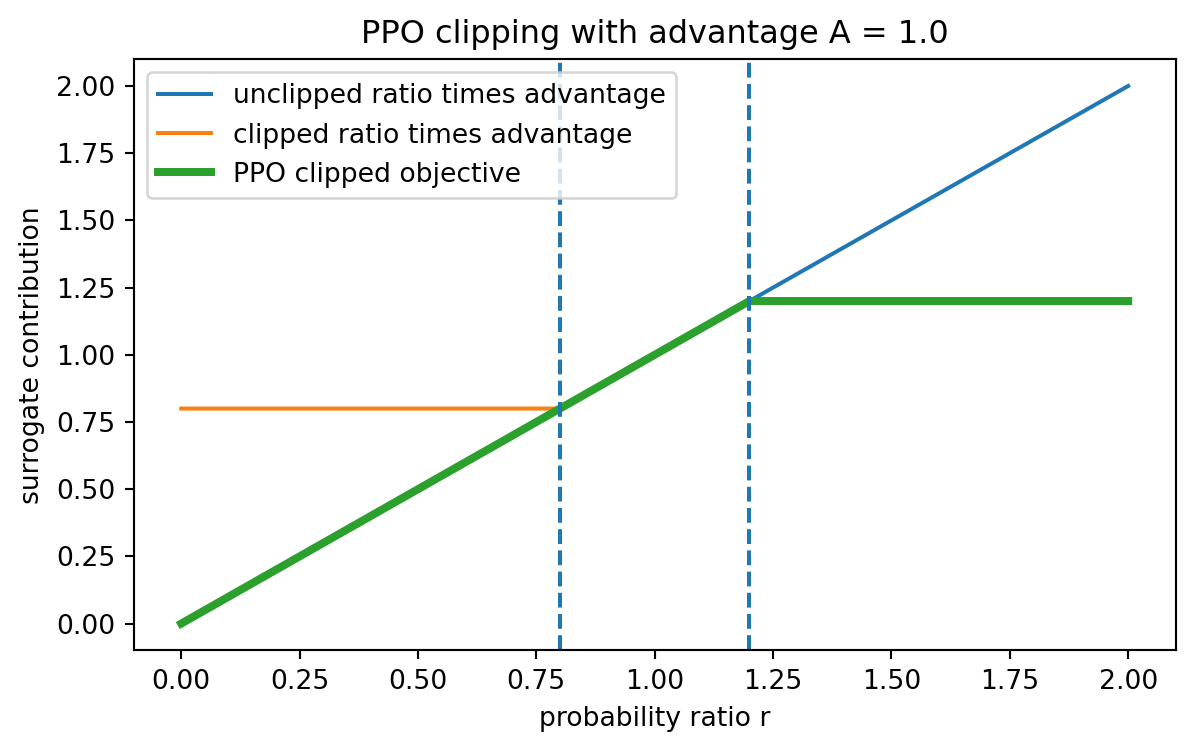
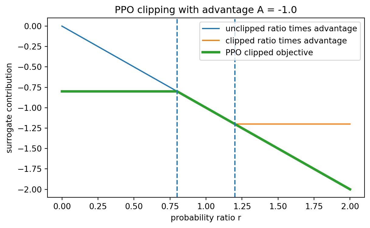
The clipping has different effects depending on the sign of the advantage.

If \(\widehat A_t>0\), increasing \(r_t(\theta)\) improves the ordinary surrogate. But PPO stops rewarding increases once

\[ r_t(\theta)>1+\epsilon. \]

If \(\widehat A_t<0\), decreasing \(r_t(\theta)\) improves the ordinary surrogate. But PPO stops rewarding decreases once

\[ r_t(\theta)<1-\epsilon. \]

Thus PPO discourages updates that change action probabilities too aggressively.

21.8.1 Interactive: PPO clipped objective

The clipped objective is piecewise linear in the probability ratio. Compare positive and negative advantages.

PPO clipping is not the same as a mathematical guarantee of monotone improvement. It is a computationally convenient surrogate that makes very large probability-ratio changes less attractive during gradient ascent.

21.9 18.8 Advantage estimation and GAE

The PPO objective requires an advantage estimate. A common choice is Generalized Advantage Estimation from Chapter 16. Define the TD residual

\[ \delta_t = R_{t+1}+\gamma V_\phi(S_{t+1})-V_\phi(S_t). \]

The GAE estimator is

\[ \widehat A_t^{\mathrm{GAE}(\gamma,\lambda)} = \sum_{k=0}^{\infty} (\gamma\lambda)^k\delta_{t+k}. \]

When \(\lambda=0\), the estimate is close to a one-step TD advantage. When \(\lambda\) is near \(1\), it uses longer returns. Thus \(\lambda\) controls a bias-variance tradeoff.

PPO commonly trains two objects:

an actor \(\pi_\theta(a\mid s)\);
a critic \(V_\phi(s)\).

A typical combined loss for minimization is

\[ \mathcal L(\theta,\phi) = -L^{\mathrm{CLIP}}(\theta) + c_v\mathbb E_t\left[(V_\phi(S_t)-\widehat R_t)^2\right] - c_e\mathbb E_t\left[H(\pi_\theta(\cdot\mid S_t))\right], \]

where \(\widehat R_t\) is a return target for the critic, \(H\) is policy entropy, and \(c_v,c_e\) are tuning constants.

21.10 18.9 Python example: PPO clipping

The following code computes the clipped PPO objective for positive and negative advantages.

import numpy as np
import matplotlib.pyplot as plt

ratios = np.linspace(0.0, 2.0, 401)
eps = 0.2

for A in [1.0, -1.0]:
    unclipped = ratios * A
    clipped = np.clip(ratios, 1 - eps, 1 + eps) * A
    ppo_objective = np.minimum(unclipped, clipped)

    plt.figure(figsize=(7, 4))
    plt.plot(ratios, unclipped, label="unclipped ratio times advantage")
    plt.plot(ratios, clipped, label="clipped ratio times advantage")
    plt.plot(ratios, ppo_objective, linewidth=3, label="PPO clipped objective")
    plt.axvline(1 - eps, linestyle="--")
    plt.axvline(1 + eps, linestyle="--")
    plt.title(f"PPO clipping with advantage A = {A}")
    plt.xlabel("probability ratio r")
    plt.ylabel("surrogate contribution")
    plt.legend()
    plt.show()

The graph shows why the minimum is used. For positive advantages, the objective is capped above when the ratio becomes too large. For negative advantages, the objective is capped when the ratio becomes too small.

21.11 18.10 Python example: softmax policy ratios and KL divergence

For a finite action space, a softmax policy can be written as

\[ \pi_\theta(a\mid s) = \frac{\exp(z_\theta(s,a))}{\sum_b \exp(z_\theta(s,b))}. \]

The next code compares an old and a new action distribution.

import numpy as np

np.set_printoptions(precision=4, suppress=True)

def softmax(logits):
    x = np.asarray(logits, dtype=float)
    x = x - np.max(x)
    e = np.exp(x)
    return e / e.sum()

def kl_divergence(p, q):
    p = np.asarray(p, dtype=float)
    q = np.asarray(q, dtype=float)
    return np.sum(p * (np.log(p + 1e-12) - np.log(q + 1e-12)))

old_logits = np.array([0.2, 0.0, -0.3])
new_logits = np.array([0.5, -0.1, -0.4])

old_policy = softmax(old_logits)
new_policy = softmax(new_logits)
ratios = new_policy / old_policy

print("old policy:", old_policy)
print("new policy:", new_policy)
print("probability ratios:", ratios)
print("KL(old || new):", kl_divergence(old_policy, new_policy))

old policy: [0.4123 0.3376 0.2501]
new policy: [0.5114 0.2807 0.2079]
probability ratios: [1.2403 0.8314 0.8314]
KL(old || new): 0.019715218752281924

A policy update is small when the ratios are close to \(1\) and the KL divergence is small.

21.12 18.11 Python example: a two-action bandit PPO update

A multi-armed bandit is the simplest policy optimization problem. There is one state and several actions. The objective is the expected reward under the current action distribution.

For a two-action softmax policy with logits \(\theta=(\theta_0,\theta_1)\),

\[ \pi_\theta(a) = \frac{\exp(\theta_a)}{\exp(\theta_0)+\exp(\theta_1)}. \]

The following code implements a small PPO-style update using sampled actions and rewards.

import numpy as np

rng = np.random.default_rng(7243)

reward_means = np.array([0.0, 1.0])
theta = np.array([0.0, 0.0])
learning_rate = 0.25
eps_clip = 0.2
batch_size = 200
num_updates = 40

def softmax_np(logits):
    z = logits - np.max(logits)
    e = np.exp(z)
    return e / e.sum()

def grad_log_softmax(probs, action):
    grad = -probs.copy()
    grad[action] += 1.0
    return grad

history = []

for update in range(num_updates):
    old_theta = theta.copy()
    old_probs = softmax_np(old_theta)

    actions = rng.choice(2, size=batch_size, p=old_probs)
    rewards = reward_means[actions] + 0.25 * rng.normal(size=batch_size)
    baseline = rewards.mean()
    advantages = rewards - baseline

    grad = np.zeros_like(theta)
    new_probs = softmax_np(theta)

    for action, adv in zip(actions, advantages):
        ratio = new_probs[action] / old_probs[action]
        clipped_ratio = np.clip(ratio, 1 - eps_clip, 1 + eps_clip)

        # Gradient is active only where the minimum selects the unclipped term.
        use_unclipped = (ratio * adv) <= (clipped_ratio * adv)
        if use_unclipped:
            grad += adv * ratio * grad_log_softmax(new_probs, action)

    theta += learning_rate * grad / batch_size
    probs = softmax_np(theta)
    expected_reward = np.dot(probs, reward_means)
    history.append((update, probs[0], probs[1], expected_reward))

history = np.array(history)
print("final theta:", theta)
print("final policy:", softmax_np(theta))
print("final expected reward:", history[-1, 3])

final theta: [-1.3494  1.3494]
final policy: [0.063 0.937]
final expected reward: 0.9369512362587206

This is not a production PPO implementation. It is a minimal mathematical laboratory: it shows how ratios, advantages, clipping, and stochastic-gradient updates interact.

21.12.1 Interactive: Bandit policy optimization

This figure shows typical learning trajectories for a two-action bandit under different update sizes.

21.13 18.12 Continuous actions and Gaussian policies

In continuous control, a common policy is Gaussian:

\[ \pi_\theta(a\mid s) = \mathcal N(a;\mu_\theta(s),\sigma_\theta^2(s)). \]

For a one-dimensional Gaussian with fixed standard deviation \(\sigma\), the log-density is

\[ \log \pi_\theta(a\mid s) = -\frac{1}{2}\log(2\pi\sigma^2) -\frac{(a-\mu_\theta(s))^2}{2\sigma^2}. \]

If only the mean is parameterized, then

\[ \nabla_\theta\log \pi_\theta(a\mid s) = \frac{a-\mu_\theta(s)}{\sigma^2} \nabla_\theta\mu_\theta(s). \]

This formula explains a basic continuous-action policy-gradient intuition: actions above the current mean increase the mean if their advantage is positive and decrease it if their advantage is negative.

21.13.1 Interactive: Gaussian policy update

The plot shows how changing the mean of a Gaussian policy affects likelihood ratios for sampled actions.

21.14 18.13 PPO with early stopping by KL

Many PPO implementations use clipping and also monitor KL divergence. If the empirical KL becomes too large, training on the current batch stops early.

A simple diagnostic is

\[ \widehat D_{\mathrm{KL}} \approx \frac{1}{n}\sum_{i=1}^n \left( \log \pi_{\theta_{\text{old}}}(a_i\mid s_i) - \log \pi_\theta(a_i\mid s_i) \right). \]

The estimate is computed on samples from the old policy. Large values mean the new policy is moving too far from the data-collection policy.

21.14.1 Interactive: PPO epochs and early stopping

Repeated optimization epochs can improve the surrogate objective but also increase KL divergence. This figure illustrates the diagnostic tradeoff.

21.15 18.14 Practical PPO objective

A practical PPO loss often combines three terms:

\[ \mathcal L = \mathcal L_{\mathrm{policy}} + c_v\mathcal L_{\mathrm{value}} + c_e\mathcal L_{\mathrm{entropy}}. \]

For minimization, the policy term is usually the negative of the clipped objective:

\[ \mathcal L_{\mathrm{policy}} = - \mathbb E_t \left[ \min \left( r_t(\theta)\widehat A_t, \operatorname{clip}(r_t(\theta),1-\epsilon,1+\epsilon)\widehat A_t \right) \right]. \]

The value loss is often

\[ \mathcal L_{\mathrm{value}} = \mathbb E_t \left[ (V_\phi(S_t)-\widehat R_t)^2 \right], \]

and the entropy term is often written with a negative sign because we want to maximize entropy:

\[ \mathcal L_{\mathrm{entropy}} = - \mathbb E_t \left[ H(\pi_\theta(\cdot\mid S_t)) \right]. \]

PPO training template

Collect trajectories using the current policy \(\pi_{\theta_{\text{old}}}\).
Estimate returns \(\widehat R_t\) and advantages \(\widehat A_t\).
Normalize advantages within the batch.
For several epochs, update \(\theta\) using the clipped surrogate.
Update the critic parameters \(\phi\) using a value loss.
Monitor approximate KL divergence, entropy, value loss, and average return.
Set \(\theta_{\text{old}}\leftarrow\theta\) and collect new data.

21.16 18.15 What can go wrong?

Policy optimization is powerful but delicate. Common failure modes include:

Advantage scale problems. Large or poorly normalized advantages can create unstable updates.
Too many epochs on old data. The ratio \(r_t(\theta)\) becomes unreliable when the new policy moves far from the old policy.
Critic error. Bad value estimates lead to bad advantage estimates.
Entropy collapse. The policy becomes nearly deterministic too early.
Reward scaling. Large rewards can cause large gradients.
Hidden implementation errors. Old log-probabilities, new log-probabilities, and advantages must correspond to the same sampled state-action pairs.

A useful diagnostic set is:

\[ \text{average return}, \quad \text{policy loss}, \quad \text{value loss}, \quad \text{entropy}, \quad \text{KL divergence}, \quad \text{clip fraction}. \]

The clip fraction is the fraction of samples for which \(r_t(\theta)\) lies outside \([1-\epsilon,1+\epsilon]\).

21.17 18.16 AI-assisted learning components

AI prompt: derive the PPO objective

Ask an AI assistant:

Starting from the surrogate objective \(\mathbb E_t[r_t(\theta)\widehat A_t]\), explain why PPO replaces it by a clipped surrogate. Discuss separately the cases \(\widehat A_t>0\) and \(\widehat A_t<0\).

Then check whether the explanation correctly identifies which probability-ratio changes are discouraged.

AI prompt: audit policy-ratio code

Give an AI assistant a PPO implementation and ask:

Check whether the code stores old log-probabilities at data-collection time and uses them consistently when computing \(r_t(\theta)=\exp(\log\pi_\theta-\log\pi_{\theta_{\text{old}}})\). Identify any data leakage or recomputation mistake.

This is a common source of silent PPO bugs.

AI prompt: compare TRPO and PPO

Ask:

Compare TRPO and PPO from the viewpoint of constrained optimization. Which method uses an explicit KL constraint, and which uses a clipped surrogate? What mathematical guarantee is lost when moving from TRPO to PPO?

21.18 18.17 Summary

Policy optimization treats the policy as the object to be optimized. The main mathematical ingredients are:

a parameterized stochastic policy \(\pi_\theta(a\mid s)\);
a trajectory objective \(J(\theta)\);
likelihood-ratio gradients;
advantage functions;
importance ratios \(r_t(\theta)\);
KL divergence as a measure of policy movement;
trust-region and proximal surrogate objectives;
actor-critic estimation of advantages and values.

TRPO uses a constrained optimization viewpoint. PPO replaces the hard trust-region constraint with a clipped objective that is easier to implement and optimize. Both methods reflect the same principle: policy-gradient steps should improve the policy without moving it too far from the distribution that generated the data.

21.19 Exercises

21.19.1 Conceptual exercises

Explain why policy optimization is especially natural for continuous action spaces.
Why does the state distribution change when the policy changes?
Explain the role of the advantage estimate \(\widehat A_t\) in PPO.
Why is the probability ratio \(r_t(\theta)\) more useful than the raw probability \(\pi_\theta(A_t\mid S_t)\)?
Explain why PPO can reuse a batch for several epochs but should not reuse it indefinitely.

21.19.2 Mathematical exercises

Starting from the trajectory density \(p_\theta(\tau)\), derive the likelihood-ratio policy-gradient identity.
Prove that if \(\theta=\theta_{\text{old}}\), then \(r_t(\theta)=1\) for every sampled state-action pair.
For a two-action policy \(p=(p,1-p)\) and \(q=(q,1-q)\), compute \(D_{\mathrm{KL}}(p\Vert q)\) explicitly.
For \(\widehat A>0\), write the PPO clipped objective as a piecewise function of \(r\). Repeat for \(\widehat A<0\).
Let \(\pi_\theta\) be a Gaussian policy with fixed variance. Derive \(\nabla_\theta\log\pi_\theta(a\mid s)\) when \(\mu_\theta(s)=\theta^Tx(s)\).

21.19.3 Computational exercises

Implement the PPO clipped objective for a vector of ratios and advantages.
Simulate two categorical policies and compute empirical ratios and KL divergence.
Modify the bandit PPO example by changing the clipping parameter \(\epsilon\). Plot the final action probabilities.
Add entropy regularization to the bandit example and compare learning curves.
Implement an early-stopping rule based on approximate KL divergence.

21.19.4 AI-assisted exercises

Ask an AI assistant to explain PPO clipping. Then identify whether it correctly treats positive and negative advantages.
Ask an AI assistant to generate pseudocode for PPO. Check whether it stores old log-probabilities before updating the policy.
Ask an AI assistant to compare natural policy gradient, TRPO, and PPO. Rewrite the answer using precise mathematical notation.
Ask an AI assistant to inspect a PPO training log with return, entropy, KL, and clip fraction. Identify likely failure modes.

21.20 Notes for instructors

This chapter is a natural bridge from policy-gradient theory to modern deep RL. For MA Applied Math students, emphasize constrained optimization, KL geometry, and natural gradients. For MS Statistics students, emphasize importance ratios, distribution shift, variance, and diagnostic estimation. A good lecture sequence is:

policy objective and likelihood-ratio gradient;
surrogate objective using old-policy data;
performance difference lemma;
KL trust region and natural gradient;
PPO clipping and diagnostics;
small Python bandit experiment.