Core idea. A Markov decision process is a Markov reward process with choices. At each state the agent selects an action, and the selected action changes both the next-state distribution and the reward distribution. Once a policy is fixed, the MDP reduces to the Markov reward process of Chapter sec-ch03-markov-reward-processes. Optimizing over policies is the beginning of reinforcement learning control.
The central object is
\[
(\mathcal S,\mathcal A,P,r,\gamma),
\]
with transition law
\[
P(s'\mid s,a)=P(S_{t+1}=s'\mid S_t=s,A_t=a)
\]
and expected reward
\[
r(s,a)=\mathbb E[R_{t+1}\mid S_t=s,A_t=a].
\]
7.1 Learning goals
After reading this chapter, students should be able to:
define a finite discounted Markov decision process precisely;
distinguish states, actions, transition laws, reward models, policies, and trajectories;
explain the Markov property in a controlled stochastic system;
distinguish deterministic, randomized, stationary, nonstationary, Markov, and history-dependent policies;
derive the policy-induced transition matrix \(P_\pi\) and reward vector \(r_\pi\);
show how a fixed policy turns an MDP into an MRP;
define \(V^\pi\), \(Q^\pi\), \(V^*\), and \(Q^*\) for an MDP;
compute policy values in a small MDP using linear algebra and Python;
connect MDP modeling to AI-assisted problem formulation and modern reinforcement learning.
7.2 4.1 Why MDPs are the mathematical core of reinforcement learning
Chapters sec-markov-chains-review and sec-ch03-markov-reward-processes studied stochastic systems with no decisions. A Markov chain describes random state evolution. A Markov reward process adds numerical rewards. A Markov decision process adds actions.
In a Markov reward process, the transition probability from \(s\) to \(s'\) is simply
\[
P(s'\mid s).
\]
In a Markov decision process, the transition probability depends on the action:
\[
P(s'\mid s,a).
\]
This apparently small change is fundamental. It turns evaluation into optimization. The agent is no longer only asking:
What is the expected future reward of this stochastic process?
It is now asking:
Which decision rule creates the stochastic process with the largest expected future reward?
A policy chooses actions. The environment responds stochastically. The resulting state sequence is a Markov chain only after the policy has been specified. This separation is one of the cleanest ways to understand the whole book:
Dynamic programming assumes the MDP model is known and optimizes exactly or approximately. Reinforcement learning uses data generated by interaction to estimate values, improve policies, or learn a model.
An MDP separates modeling from decision making. The model says what can happen after each state-action pair. The policy says what the agent chooses to do.
Both descriptions are equivalent for value calculations when only expected discounted return is optimized. Transition-based rewards can be more natural when the reward depends on the realized next state, such as receiving a penalty only when the system fails.
7.3.1 Controlled Markov property
The controlled Markov property says that, conditional on the current state and current action, the distribution of the next state and reward does not depend on the earlier history:
\[
P(S_{t+1}=s',R_{t+1}\in B
\mid S_0,A_0,R_1,\ldots,S_t=s,A_t=a)
=
P(S_{t+1}=s',R_{t+1}\in B\mid S_t=s,A_t=a).
\]
The current state \(S_t\) must therefore contain all information from the past that is needed for predicting the next transition, once the action is known. This is a modeling assumption. In practice, building a useful state representation is often as important as choosing an algorithm.
Modeling principle. If the future depends on a feature of the past that is not included in \(S_t\), then the process may not be Markov in the chosen state variable. A common fix is to enlarge the state so that it includes enough history or sufficient statistics.
7.4 4.3 Running example: study-planning MDP
We use a small study-planning example throughout this chapter. The state space is
The action Consolidate emphasizes review, repetition, and stability. The action Challenge emphasizes harder problems, faster movement toward mastery, but also higher risk of confusion.
For a fixed ordering of states \([\text{Review},\text{Practice},\text{Mastery}]\), define the transition matrices
The challenge action has lower reward in Review because it may be frustrating before the foundations are secure, but it has higher reward in Practice and Mastery because it can accelerate progress.
The interactive network shows the two transition kernels side by side. An MDP is not one transition matrix; it is a collection of transition matrices indexed by actions.
7.5 4.4 Policies
A policy is a rule for choosing actions. Policies may be classified by how much information they use and whether they randomize.
This policy consolidates at Review but chooses challenge later.
If every state has two actions and there are \(m\) states, then there are \(2^m\) deterministic stationary policies. More generally, if state \(s\) has \(|\mathcal A(s)|\) feasible actions, the number of deterministic stationary policies is
\[
\prod_{s\in\mathcal S}|\mathcal A(s)|.
\]
For small MDPs, enumeration may be possible. For large state spaces, direct enumeration is impossible.
7.5.2 Randomized stationary policies
A randomized stationary policy assigns a probability distribution over actions at each state:
The display above shows how changing the probability of choosing Challenge at each state changes the policy. Randomization is not merely a technicality. It is the mathematical form of exploration, mixed strategies, entropy-regularized control, and differentiable policy optimization.
7.5.3 Nonstationary and history-dependent policies
A nonstationary Markov policy may depend on time:
\[
\pi_t(a\mid s)=P(A_t=a\mid S_t=s).
\]
A history-dependent policy may depend on the whole past:
\[
\pi_t(a\mid h_t),
\]
where
\[
h_t=(S_0,A_0,R_1,S_1,A_1,R_2,\ldots,S_t).
\]
History-dependent policies are mathematically general, but for many finite discounted MDPs one can restrict attention to stationary deterministic policies when optimizing expected discounted reward. This is a deep and useful fact from MDP theory (puterman1994markov?).
For discounted finite MDPs with known model, optimal stationary deterministic policies exist. Modern reinforcement learning often still uses randomized policies because they support exploration, regularization, and gradient-based optimization.
7.6 4.5 A fixed policy induces an MRP
The most important calculation in this chapter is the reduction from an MDP to an MRP. Fix a randomized stationary policy \(\pi\). The policy-induced transition matrix is
The mixture happens row by row because the action is chosen after observing the current state.
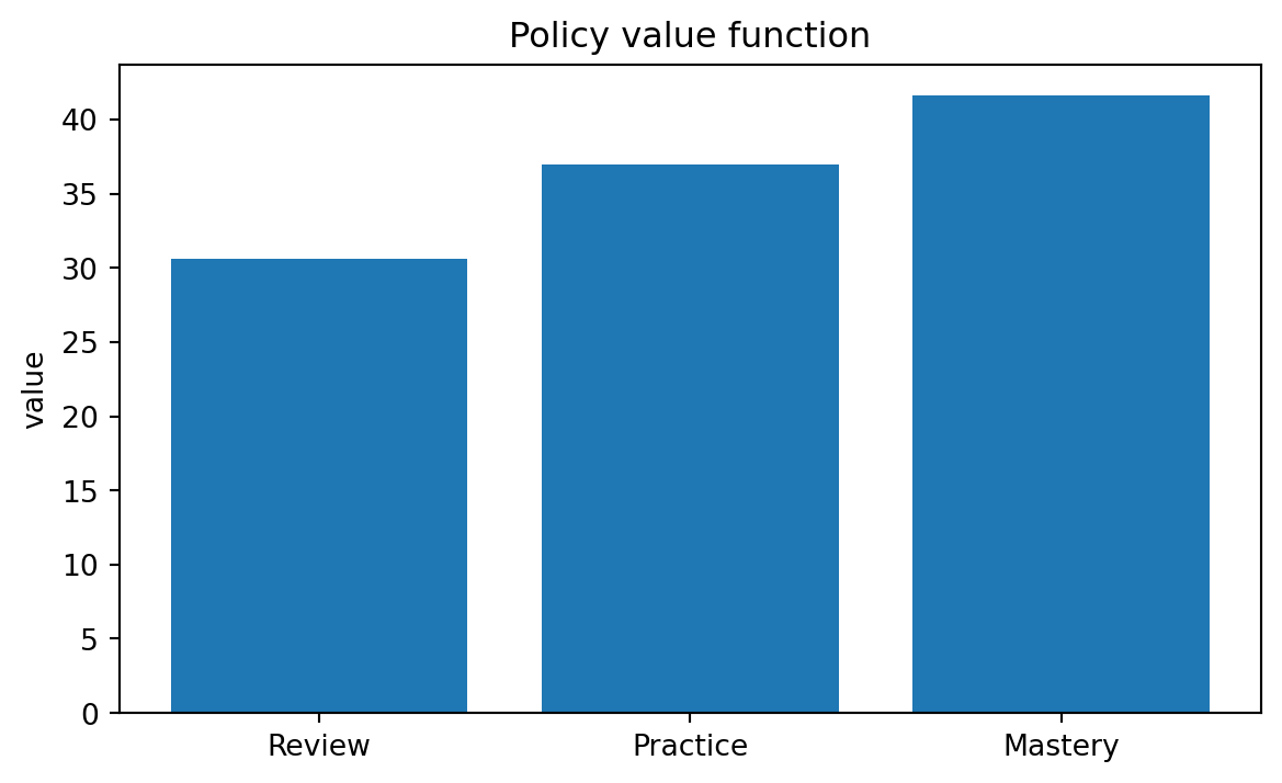
The interactive visualization shows how values change as the probability of choosing Challenge changes. This is a small example of a central RL idea: changing the policy changes both immediate rewards and future state distributions.
Later chapters show that they satisfy Bellman optimality equations. For now, the key point is that \(Q^\pi\) tells us how good a one-step deviation is before returning to policy \(\pi\).
Therefore \(V^\pi\) is the unique fixed point of \(T^\pi\).
Policy evaluation theorem for finite discounted MDPs. Fix a stationary randomized policy \(\pi\) in a finite MDP with \(0\leq\gamma<1\). Then \(V^\pi\) exists, is unique, and satisfies
\[
V^\pi=(I-\gamma P_\pi)^{-1}r_\pi.
\]
Proof. Since \(P_\pi\) is a stochastic matrix, its induced sup-norm operator norm satisfies \(\|P_\pi\|_\infty=1\). Thus
measures whether Challenge is a better one-step action than Consolidate when future behavior follows \(\pi\). This quantity is the first appearance of the policy improvement idea developed in Chapter 7.
Not every decision problem is naturally infinite horizon. A course lasts a semester, a clinical trial has a planned endpoint, and an inventory problem may have a finite planning period. In a finite-horizon MDP, the objective is
Finite-horizon value functions depend on time. Let \(V_t(s)\) be the optimal expected reward from time \(t\) to the horizon \(T\), given \(S_t=s\). The terminal condition is
Finite-horizon problems naturally produce nonstationary policies. The best action near the end of the horizon may differ from the best action early in the horizon.
The plot shows how optimal values change as the remaining horizon increases. Short horizons emphasize immediate reward. Longer horizons give the transition dynamics more time to matter.
This computation is the finite-horizon version of dynamic programming. Infinite-horizon value iteration in Chapter 8 can be understood as repeatedly applying a time-homogeneous version of this recursion.
7.11 4.10 Occupancy measures
Value functions are one way to describe an MDP under a policy. Occupancy measures are another. They are especially useful in statistical learning theory, offline RL, and policy gradient methods.
For an initial distribution \(\mu\), define the discounted state occupancy measure of policy \(\pi\) by
This identity is important because it converts a sequential objective into an expectation with respect to a policy-dependent distribution.
Occupancy measures explain why data distribution matters in reinforcement learning. A policy only generates data from the states and actions it visits often. If an offline dataset has poor coverage of important actions, value estimates can be unreliable.
mu = np.array([1.0, 0.0, 0.0])occupancy = (1- gamma) * mu @ np.linalg.inv(np.eye(3) - gamma * P_pi)pd.DataFrame({"state": states,"discounted occupancy": occupancy})
state
discounted occupancy
0
Review
0.416857
1
Practice
0.285640
2
Mastery
0.297503
7.12 4.11 Model-based and model-free viewpoints
An MDP model contains \(P\) and \(r\). If these are known, the agent can plan. If they are unknown, the agent must learn from samples.
and then uses dynamic programming or planning on the estimated model. This approach makes the probabilistic structure explicit and is natural for students trained in statistics.
7.12.2 Model-free viewpoint
The model-free approach estimates values or policies directly, without explicitly estimating \(P\). For example, Q-learning estimates \(Q^*\) from sampled transitions
\[
(S_t,A_t,R_{t+1},S_{t+1}).
\]
The distinction is not absolute. Many modern algorithms combine model learning, value learning, policy learning, and simulation.
The MDP is the mathematical object, not necessarily the algorithm. Algorithms differ in whether they use the model explicitly, estimate it, or avoid representing it directly.
7.13 4.12 Statistical modeling issues
For MA Applied Math and MS Statistics students, the MDP definition should raise several modeling questions.
7.13.1 What is the state?
The state should contain enough information to make the future conditionally independent of the past, given the current action. In practice, this may require feature engineering, filtering, embeddings, or belief states.
For example, in a tutoring system, the current quiz score alone may not be Markov. The student’s history of misconceptions, time since last review, and previous activities may be needed.
7.13.2 What is the reward?
Reward design is a modeling decision. A poorly chosen reward can produce undesirable behavior. For example, a tutoring system rewarded only for short-term engagement might avoid difficult but important material.
Mathematically, reward design specifies the objective function. A change in reward is a change in the optimization problem.
7.13.3 What is the action space?
The action space determines what the agent is allowed to choose. Too small an action space may exclude useful decisions. Too large an action space may make learning statistically and computationally difficult.
7.13.4 Is the Markov assumption reasonable?
The Markov assumption is not automatically true. It is a statement about the chosen representation. When it fails, one may consider:
enlarging the state with lagged variables;
using recurrent models or sequence models;
estimating a belief state;
formulating a partially observable MDP;
accepting an approximate Markov model for tractability.
These modeling choices connect reinforcement learning to statistics, stochastic processes, causal inference, and AI systems.
7.14 4.13 AI-assisted learning component
Generative AI tools can help students learn MDP modeling, but the mathematical specification must remain explicit. A useful workflow is:
describe the real decision problem in words;
ask the AI tool to identify possible states, actions, rewards, and transition uncertainties;
translate the suggestions into a precise MDP definition;
check whether the proposed state is plausibly Markov;
write down \(P(s'\mid s,a)\) and \(r(s,a)\) for a small finite version;
compute \(P_\pi\), \(r_\pi\), and \(V^\pi\) by hand or in Python;
critique the reward and state representation.
7.14.1 Prompt template
A useful prompt is:
I am modeling a finite Markov decision process for [application]. Propose a small state space, action space, transition model, and reward function. Then explain which parts of the state are needed for the Markov property. Keep the example small enough that I can compute policy evaluation by hand.
7.14.2 Verification questions
After receiving an AI-generated model, students should ask:
Are the transition probabilities nonnegative and do they sum to one for each state-action pair?
Is the reward function aligned with the real objective?
Does the state contain enough information for the Markov property?
Are any actions infeasible in some states?
Does the model confuse correlation with causation?
Can I compute \(P_\pi\) and \(r_\pi\) from the proposed policy?
7.14.3 AI debugging exercise
Ask an AI tool to write Python code for policy evaluation in the study-planning MDP. Then check whether it:
mixes rows of \(P^C\) and \(P^H\) using the state-specific action probabilities;
computes \(r_\pi\) consistently with the policy;
solves \((I-\gamma P_\pi)V=r_\pi\) rather than using elementwise division;
distinguishes \(V^\pi\) from \(Q^\pi\).
The goal is not to trust the AI output. The goal is to use mathematical structure to audit it.
7.15 4.14 Summary
This chapter introduced the finite discounted Markov decision process. The key ideas are:
an MDP adds actions to a Markov reward process;
the transition law is \(P(s'\mid s,a)\), not merely \(P(s'\mid s)\);
a policy specifies how actions are chosen;
a fixed policy induces a Markov reward process with
finite-horizon MDPs are solved by backward induction;
occupancy measures describe the distribution of states and actions generated by a policy;
MDP modeling requires careful choices of state, action, reward, and transition structure.
The next chapter studies Bellman equations in greater depth and introduces optimality equations.
7.16 Exercises
7.16.1 Conceptual exercises
Explain why a Markov decision process is not the same thing as a Markov chain.
Give an example of a state representation that is not Markov. Then enlarge it to make it closer to Markov.
Explain why randomized policies are useful even though deterministic optimal policies exist for many finite discounted MDPs.
In your own words, explain the statement: an MDP plus a policy equals an MRP.
Describe a real decision problem in education, finance, health, or operations. Identify possible states, actions, rewards, and transition uncertainties.
7.16.2 Mathematical exercises
Let \(\pi\) be a randomized stationary policy. Prove that \(P_\pi\) is a row-stochastic matrix.
Derive the Bellman expectation equation for \(V^\pi\) from the recursive identity \(G_t=R_{t+1}+\gamma G_{t+1}\).
Show that
\[
V^\pi(s)=\sum_a\pi(a\mid s)Q^\pi(s,a).
\]
For the study-planning MDP, compute \(P_\pi\) and \(r_\pi\) by hand for the policy that always chooses Challenge.
For the same MDP, compute \(P_\pi\) and \(r_\pi\) for the deterministic policy that chooses Consolidate in Review and Challenge otherwise.
Prove that \(T^\pi\) is a contraction in the sup norm.
Let \(\mu\) be an initial distribution. Prove that the normalized discounted occupancy measure satisfies \(\sum_s d_\mu^\pi(s)=1\).
7.16.3 Computational exercises
Modify the Python example so that \(\gamma=0.50\), \(0.90\), and \(0.99\). Compare the value functions.
Enumerate all deterministic stationary policies in the three-state, two-action study MDP. Which policy has the largest value from Review?
Estimate \(P_\pi\) by simulating 10,000 transitions under the randomized policy. Compare the empirical transition matrix with the exact one.
Compute the state-action occupancy measure \(d_\mu^\pi(s,a)\) for the study MDP.
Implement finite-horizon backward induction with a different terminal reward. How does the optimal policy change?
Construct your own three-state, two-action MDP and compute \(V^\pi\) and \(Q^\pi\) for two different policies.
7.16.4 AI-assisted exercises
Ask an AI tool to propose a small MDP for course advising. Convert the response into a precise tuple \((\mathcal S,\mathcal A,P,r,\gamma)\).
Ask the AI tool to explain why the proposed state is Markov. Critique the explanation.
Ask the AI tool to generate Python code for computing \(P_\pi\). Check whether each row sums to one.
Ask the AI tool to propose a reward function for the same MDP. Identify at least two possible unintended incentives.
Ask the AI tool to produce a deterministic policy and a randomized policy. Compute and compare their values.
7.17 Instructor notes
This chapter should be taught as the bridge from stochastic processes to decision making. Students who understand Chapters 2 and 3 should see Chapter 4 as a minimal but powerful extension: actions index transition matrices and reward vectors. The most important algebraic formula is
because it explains why policy evaluation is an MRP problem. Emphasize that MDP modeling is not automatic: the state representation, reward function, and action space are scientific modeling choices.