27  Connections to Control Theory

Core idea: reinforcement learning and optimal control study the same mathematical question: how should decisions be chosen over time when present actions affect future states? Control theory usually begins with a model of the dynamics, while reinforcement learning often begins with data generated by interaction. The common language is dynamic programming, value functions, Bellman equations, and stochastic optimization.

27.1 Learning goals

After reading this chapter, students should be able to:

• formulate deterministic and stochastic control problems as sequential optimization problems;
• derive dynamic programming recursions for controlled dynamical systems;
• solve the linear-quadratic regulator problem using Riccati recursions;
• interpret the Riccati equation as a Bellman equation for a quadratic value function;
• explain the relation between Hamilton-Jacobi-Bellman equations and continuous-time reinforcement learning;
• compare model predictive control and reinforcement learning;
• implement small LQR, Riccati, HJB, and MPC examples in Python;
• use AI tools responsibly to check derivations, dimensions, and modeling assumptions.

27.2 24.1 Why control theory belongs in reinforcement learning

Reinforcement learning is often introduced through Markov decision processes. Control theory is often introduced through dynamical systems. At first they appear different:

Reinforcement learning language	Control theory language
state \(s\)	state \(x\)
action \(a\)	control \(u\)
reward \(r(s,a)\)	negative cost \(-c(x,u)\)
transition kernel \(P(s' \mid s,a)\)	dynamics \(x_{t+1}=f(x_t,u_t,w_t)\)
policy \(\pi(a \mid s)\)	feedback control law \(u=K(x)\) or \(u=\mu(x)\)
value function \(V^\pi(s)\)	cost-to-go or value function \(J^\mu(x)\)
Bellman equation	dynamic programming equation

The mathematical problem is the same. We observe a state, choose a decision, receive an immediate reward or cost, and move to a new state. The objective is to optimize cumulative performance over time.

In this chapter we use the control convention of minimizing cost. For a discounted infinite-horizon problem, the objective is

\[ J^\mu(x_0) = E\left[\sum_{t=0}^{\infty}\gamma^t c(X_t,U_t) \mid X_0=x_0, U_t=\mu(X_t)\right]. \]

The reinforcement learning reward convention is recovered by setting

\[ r(x,u)=-c(x,u). \]

Thus minimizing expected cost is equivalent to maximizing expected reward.

Mathematical bridge. Control theory supplies precise models and analytic structure. Reinforcement learning supplies data-driven methods when the dynamics, cost, or state representation are unknown or too complex to model exactly.

27.3 24.2 Controlled dynamical systems

A discrete-time controlled dynamical system has the form

\[ X_{t+1}=f(X_t,U_t,W_{t+1}), \]

where:

• \(X_t \in R^d\) is the state;
• \(U_t \in R^m\) is the control;
• \(W_{t+1}\) is process noise;
• \(f\) is the system dynamics.

If \(W_{t+1}\) is random, then the system induces a transition kernel

\[ P(B \mid x,u)=P(f(x,u,W_{t+1}) \in B), \]

for measurable subsets \(B\) of the state space. In this way, a stochastic control model becomes an MDP.

A feedback policy is a map

\[ \mu:S \to A, \qquad U_t=\mu(X_t). \]

A randomized feedback policy is a conditional distribution

\[ \pi(du \mid x). \]

Most classical control problems emphasize deterministic feedback policies because the model is known and the objective is often convex or quadratic. Reinforcement learning emphasizes randomized policies because exploration is necessary when the model is not known.

27.4 24.3 Dynamic programming for finite-horizon control

Consider a finite-horizon deterministic control problem:

\[ x_{t+1}=f_t(x_t,u_t), \qquad t=0,1,\ldots,T-1. \]

The cost is

\[ \sum_{t=0}^{T-1} c_t(x_t,u_t)+g(x_T), \]

where \(g\) is a terminal cost. The value function at time \(t\) is

\[ V_t(x)=\min_{u_t,\ldots,u_{T-1}} \left[\sum_{k=t}^{T-1}c_k(x_k,u_k)+g(x_T)\right]. \]

The principle of optimality gives the backward recursion

\[ V_T(x)=g(x), \]

and

\[ V_t(x)=\min_u \left\{c_t(x,u)+V_{t+1}(f_t(x,u))\right\}. \]

This is the deterministic finite-horizon Bellman equation. In the stochastic case,

\[ X_{t+1}=f_t(X_t,U_t,W_{t+1}), \]

we obtain

\[ V_t(x)=\min_u \left\{c_t(x,u)+E[V_{t+1}(f_t(x,u,W_{t+1}))]\right\}. \]

This equation is the control-theoretic version of the finite-horizon MDP recursion.

27.4.1 Interactive: finite-horizon control as value propagation

The plot shows how a terminal quadratic cost propagates backward through a simple controlled system. The shape of the value function changes as the remaining horizon increases.

27.5 24.4 Linear-quadratic regulator

The linear-quadratic regulator is the most important exactly solvable control problem. It is also one of the cleanest examples of dynamic programming.

Consider the deterministic linear system

\[ x_{t+1}=Ax_t+Bu_t, \]

where \(x_t \in R^d\) and \(u_t \in R^m\). The infinite-horizon discounted cost is

\[ J(x_0)=\sum_{t=0}^{\infty}\gamma^t \left(x_t^TQx_t+u_t^TRu_t\right), \]

where \(Q\) is positive semidefinite and \(R\) is positive definite.

The Bellman equation is

\[ V(x)=\min_u\left\{x^TQx+u^TRu+\gamma V(Ax+Bu)\right\}. \]

The key ansatz is that the optimal value function is quadratic:

\[ V(x)=x^TPx, \]

where \(P\) is symmetric positive semidefinite. Substituting this form into the Bellman equation gives

\[ x^TPx = \min_u\left\{x^TQx+u^TRu+\gamma(Ax+Bu)^TP(Ax+Bu)\right\}. \]

For fixed \(x\), the expression inside the braces is a quadratic function of \(u\). Expanding the terms that depend on \(u\) gives

\[ u(u) = u_0+u^T(R+\gamma B^TPB)u+2\gamma x^TA^TPBu. \]

Differentiating with respect to \(u\) and setting the gradient equal to zero yields

\[ (R+\gamma B^TPB)u+\gamma B^TPAx=0. \]

Therefore the optimal feedback law has the linear form

\[ u^*(x)=-Kx, \]

where

\[ K=(R+\gamma B^TPB)^{-1}\gamma B^TPA. \]

The matrix \(P\) satisfies the discounted discrete algebraic Riccati equation

\[ P = Q+ \gamma A^TPA - \gamma^2 A^TPB(R+\gamma B^TPB)^{-1}B^TPA. \]

LQR as a Bellman equation. The Riccati equation is not a separate idea from dynamic programming. It is the Bellman optimality equation after imposing the quadratic value-function form \(V(x)=x^TPx\).

27.5.1 Interactive: LQR feedback gain

The scalar system \(x_{t+1}=ax_t+bu_t\) has a quadratic cost \(qx^2+ru^2\). The figure shows how the optimal feedback gain changes as the control penalty \(r\) changes.

27.6 24.5 Finite-horizon Riccati recursion

The finite-horizon LQR problem is

\[ \min_{u_0,\ldots,u_{T-1}} \sum_{t=0}^{T-1}\left(x_t^TQx_t+u_t^TRu_t\right)+x_T^TGx_T, \]

subject to

\[ x_{t+1}=Ax_t+Bu_t. \]

Assume

\[ V_t(x)=x^TP_tx. \]

The terminal condition is

\[ P_T=G. \]

Backward induction gives

\[ K_t=(R+B^TP_{t+1}B)^{-1}B^TP_{t+1}A, \]

and

\[ P_t =Q+A^TP_{t+1}A -A^TP_{t+1}B(R+B^TP_{t+1}B)^{-1}B^TP_{t+1}A. \]

The optimal control at time \(t\) is

\[ u_t^*=-K_tx_t. \]

Notice the exact analogy with finite-horizon value iteration: one initializes a terminal value and applies a backward Bellman recursion.

27.6.1 Interactive: Riccati convergence

The plot shows the finite-horizon Riccati matrices converging toward a steady-state solution as the horizon grows.

27.7 24.6 Python example: finite-horizon LQR

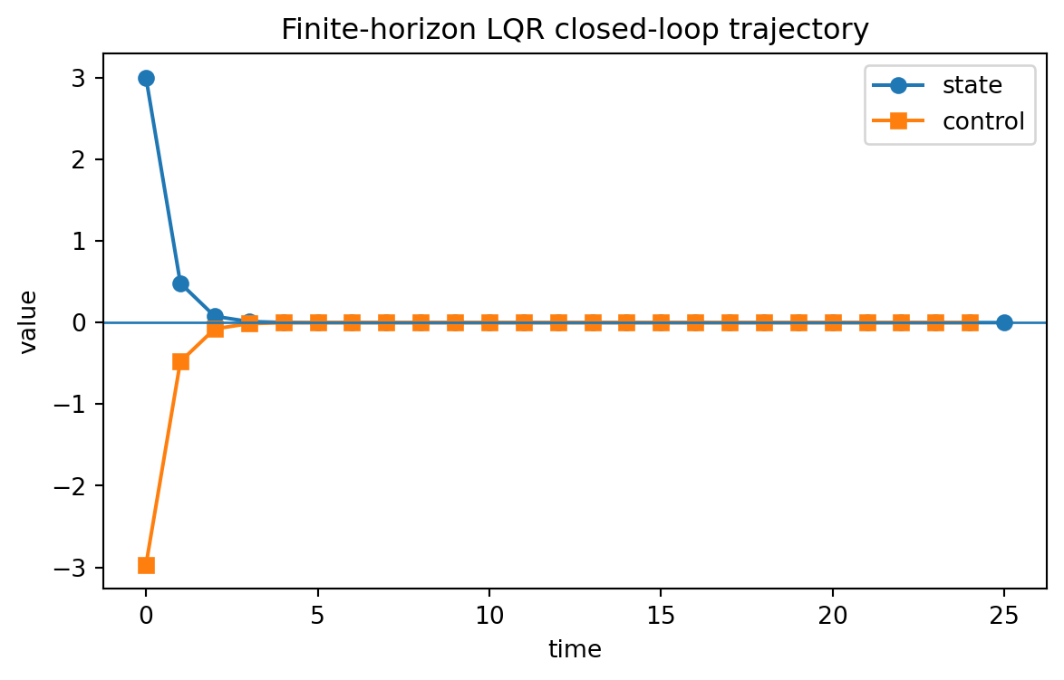
The following example solves a scalar finite-horizon LQR problem and simulates the optimal closed-loop trajectory.

import numpy as np
import matplotlib.pyplot as plt

A = np.array([[1.15]])
B = np.array([[1.0]])
Q = np.array([[1.0]])
R = np.array([[0.20]])
G = np.array([[2.0]])
T = 25

P = [None] * (T + 1)
K = [None] * T
P[T] = G.copy()

for t in range(T - 1, -1, -1):
    S = R + B.T @ P[t + 1] @ B
    K[t] = np.linalg.solve(S, B.T @ P[t + 1] @ A)
    P[t] = Q + A.T @ P[t + 1] @ A - A.T @ P[t + 1] @ B @ K[t]

x = np.zeros(T + 1)
u = np.zeros(T)
x[0] = 3.0
for t in range(T):
    u[t] = -(K[t] @ np.array([[x[t]]])).item()
    x[t + 1] = (A @ np.array([[x[t]]]) + B * u[t]).item()

plt.figure(figsize=(7, 4))
plt.plot(range(T + 1), x, marker="o", label="state")
plt.plot(range(T), u, marker="s", label="control")
plt.axhline(0, linewidth=1)
plt.xlabel("time")
plt.ylabel("value")
plt.title("Finite-horizon LQR closed-loop trajectory")
plt.legend()
plt.show()

Finite-horizon LQR trajectory for a scalar system.

The feedback gain is large at times where controlling the state strongly reduces future cost. Near the terminal time, the gain depends strongly on the terminal matrix \(G\).

27.8 24.7 Infinite-horizon LQR by value iteration

For infinite-horizon LQR, the Riccati equation can be solved by fixed-point iteration. Starting with \(P_0=0\), define

\[ P_{k+1} =Q+ \gamma A^TP_kA - \gamma^2 A^TP_kB(R+\gamma B^TP_kB)^{-1}B^TP_kA. \]

This is the LQR version of value iteration. In tabular reinforcement learning, value iteration updates a vector. In LQR, value iteration updates a matrix.

import numpy as np

A = np.array([[1.1]])
B = np.array([[1.0]])
Q = np.array([[1.0]])
R = np.array([[0.5]])
gamma = 0.95

P = np.zeros((1, 1))
history = []
for k in range(60):
    S = R + gamma * B.T @ P @ B
    K = np.linalg.solve(S, gamma * B.T @ P @ A)
    P_new = Q + gamma * A.T @ P @ A - gamma**2 * A.T @ P @ B @ np.linalg.solve(S, B.T @ P @ A)
    history.append(P_new.item())
    P = P_new

print("Approximate steady-state P:", round(P.item(), 4))
print("Approximate feedback gain K:", round(K.item(), 4))

Approximate steady-state P: 1.4433
Approximate feedback gain K: 0.8061

The closed-loop system is

\[ x_{t+1}=(A-BK)x_t. \]

The feedback gain \(K\) is useful only if it stabilizes the system. In the scalar case, stability requires

\[ |a-bK|<1. \]

In the multidimensional case, stability requires the spectral radius condition

\[ \rho(A-BK)<1. \]

27.9 24.8 Stochastic LQR and LQG

Now add process noise:

\[ X_{t+1}=AX_t+BU_t+W_{t+1}, \]

where

\[ E[W_{t+1}]=0, \qquad \operatorname{Cov}(W_{t+1})=\Sigma_W. \]

For a quadratic value function \(V(x)=x^TPx+c\), the expected next value is

\[ E[V(AX_t+BU_t+W_{t+1})] =(Ax+Bu)^TP(Ax+Bu)+\operatorname{tr}(P\Sigma_W)+c. \]

The noise term changes the value by an additive constant but does not change the optimal linear feedback gain when the noise is additive, zero-mean, and independent of the control. This is one version of the certainty-equivalence principle.

When the state is not directly observed, one obtains a linear-quadratic-Gaussian problem. The system is

\[ X_{t+1}=AX_t+BU_t+W_{t+1}, \]

and observations are

\[ Y_t=CX_t+V_t. \]

The optimal controller combines:

• a Kalman filter for estimating \(X_t\) from observations;
• an LQR controller applied to the state estimate.

This separation of estimation and control is a central result in classical control. It also foreshadows the POMDP viewpoint from Chapter 22.

27.9.1 Interactive: additive noise and expected cost

The plot compares deterministic and noisy LQR trajectories. The expected value function shifts upward under process noise, even when the feedback gain stays the same.

27.10 24.9 Continuous-time control and the HJB equation

Continuous-time deterministic control uses dynamics

\[ \frac{dX_t}{dt}=f(X_t,U_t). \]

For an infinite-horizon discounted cost

\[ J^\mu(x)=\int_0^\infty e^{-\beta t}c(X_t,U_t)dt, \]

the value function is

\[ V(x)=\inf_\mu J^\mu(x). \]

The Hamilton-Jacobi-Bellman equation is

\[ \beta V(x)=\min_u\left\{c(x,u)+\nabla V(x)^Tf(x,u)\right\}. \]

This is the continuous-time analogue of the Bellman optimality equation. The term \(\nabla V(x)^Tf(x,u)\) measures how the value changes along the controlled vector field.

For a stochastic differential equation

\[ dX_t=f(X_t,U_t)dt+\sigma(X_t,U_t)dB_t, \]

the HJB equation becomes

\[ \beta V(x)=\min_u\left\{c(x,u)+\nabla V(x)^Tf(x,u)+\frac{1}{2}\operatorname{tr}\left(\sigma\sigma^T\nabla^2V(x)\right)\right\}. \]

The second-derivative term comes from diffusion. This term is the continuous-state analogue of taking expectation over random next states.

27.10.1 Interactive: HJB discretization

The figure shows a grid approximation to a one-dimensional HJB problem. Changing the grid resolution changes the numerical approximation to the value function.

27.11 24.10 Model predictive control

Model predictive control solves a finite-horizon optimization problem at every time step. At time \(t\), it solves

\[ \min_{u_t,\ldots,u_{t+H-1}} \sum_{k=t}^{t+H-1}c(x_k,u_k)+g(x_{t+H}), \]

subject to

\[ x_{k+1}=f(x_k,u_k). \]

Only the first action \(u_t\) is applied. At the next time step the state is observed again, and the optimization problem is solved again.

This creates a feedback controller even though each optimization problem is open loop.

Model predictive control

1. Observe current state \(x_t\).
2. Solve a finite-horizon planning problem from \(x_t\).
3. Apply only the first planned control \(u_t\).
4. Observe the new state \(x_{t+1}\).
5. Repeat.

MPC and RL are connected in several ways:

• MPC uses an explicit model and online optimization.
• RL often uses offline training to learn a policy or value function.
• Model-based RL can use learned dynamics inside an MPC loop.
• Value functions can be used as terminal costs for MPC.
• MPC can generate data for imitation learning or policy distillation.

27.11.1 Interactive: MPC horizon length

The plot compares receding-horizon controllers with different planning horizons. Longer horizons usually improve control quality but increase computation.

27.12 24.11 Python example: receding-horizon control by brute force

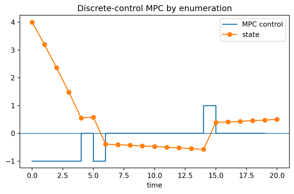
For a small scalar system with discrete controls, MPC can be implemented by enumerating all control sequences.

import itertools
import numpy as np
import matplotlib.pyplot as plt

A = 1.05
B = 1.0
controls = np.array([-1.0, 0.0, 1.0])
H = 4
T = 20
q = 1.0
r = 0.05

def rollout_cost(x0, seq):
    x = x0
    cost = 0.0
    for u in seq:
        cost += q * x**2 + r * u**2
        x = A * x + B * u
    cost += 2.0 * x**2
    return cost

def mpc_action(x):
    best_cost = np.inf
    best_u = 0.0
    for seq in itertools.product(controls, repeat=H):
        cost = rollout_cost(x, seq)
        if cost < best_cost:
            best_cost = cost
            best_u = seq[0]
    return best_u

x = np.zeros(T + 1)
u = np.zeros(T)
x[0] = 4.0
for t in range(T):
    u[t] = mpc_action(x[t])
    x[t + 1] = A * x[t] + B * u[t]

plt.figure(figsize=(7, 4))
plt.step(range(T), u, where="post", label="MPC control")
plt.plot(range(T + 1), x, marker="o", label="state")
plt.axhline(0, linewidth=1)
plt.xlabel("time")
plt.title("Discrete-control MPC by enumeration")
plt.legend()
plt.show()

This example is intentionally small. In high-dimensional systems, enumeration is impossible, and one uses numerical optimization, linearization, sampling-based planning, learned models, or approximate value functions.

27.13 24.12 RL and control: what changes when the model is unknown?

Classical control often assumes that the dynamics are known:

\[ x_{t+1}=f(x_t,u_t). \]

Reinforcement learning usually assumes that the agent can sample transitions but may not know \(f\) or \(P\) explicitly.

This creates three statistical problems.

27.13.1 Estimation

If the system is linear,

\[ X_{t+1}=AX_t+BU_t+W_{t+1}, \]

then \(A\) and \(B\) can be estimated by least squares from data. Define

\[ Z_t= \begin{bmatrix} X_t \\ U_t \end{bmatrix}, \qquad X_{t+1}=\Theta Z_t+W_{t+1}, \]

where

\[ \Theta=[A \ B]. \]

The least-squares estimator is

\[ \widehat{\Theta} = \left(\sum_t X_{t+1}Z_t^T\right) \left(\sum_t Z_tZ_t^T\right)^{-1}. \]

This is model learning.

27.13.2 Exploration

Good estimation requires exciting the system. If the controller always drives the state to zero quickly, the data may not identify all directions of the dynamics. Thus control and estimation are coupled.

27.13.3 Robustness

A controller designed for an estimated model may perform poorly if the estimate is wrong. Robust control and safe RL study how to optimize performance while controlling model error.

27.13.4 Interactive: model estimation and control performance

The plot shows how uncertainty in the learned dynamics affects the closed-loop cost of an LQR-style controller.

27.14 24.13 Python example: estimating a linear system

The next example estimates a scalar linear system from exploratory data and then computes an LQR gain for the estimated model.

import numpy as np

rng = np.random.default_rng(7243)
T = 400
true_a = 1.08
true_b = 0.75
noise_sd = 0.15

x = np.zeros(T + 1)
u = rng.normal(0, 1.0, size=T)
x[0] = 0.5
for t in range(T):
    x[t + 1] = true_a * x[t] + true_b * u[t] + rng.normal(0, noise_sd)

Z = np.column_stack([x[:-1], u])
y = x[1:]
theta_hat, *_ = np.linalg.lstsq(Z, y, rcond=None)
a_hat, b_hat = theta_hat

print("Estimated a:", round(a_hat, 3), "true a:", true_a)
print("Estimated b:", round(b_hat, 3), "true b:", true_b)

# Scalar Riccati iteration for estimated dynamics
q, r, gamma = 1.0, 0.3, 0.95
P = 0.0
for _ in range(100):
    P = q + gamma * a_hat**2 * P - (gamma**2 * a_hat**2 * b_hat**2 * P**2) / (r + gamma * b_hat**2 * P)
K_hat = (gamma * b_hat * P * a_hat) / (r + gamma * b_hat**2 * P)

print("Estimated LQR gain:", round(K_hat, 3))
print("Closed-loop scalar coefficient:", round(a_hat - b_hat * K_hat, 3))

Estimated a: 1.08 true a: 1.08
Estimated b: 0.746 true b: 0.75
Estimated LQR gain: 1.041
Closed-loop scalar coefficient: 0.304

This is the simplest model-based RL pipeline:

\[ \text{data} \to \widehat{f} \to \widehat{\mu}. \]

The difficulty is that each arrow introduces approximation and statistical error.

27.15 24.14 Control-theoretic view of value functions

In RL, we often define a value function as an expected return. In control, the value function also has geometric meaning. It measures how costly it is to be at a given state.

For LQR,

\[ V(x)=x^TPx. \]

The level sets

\[ \{x:x^TPx=c\} \]

are ellipsoids. Directions with large curvature in \(P\) are costly directions. The optimal feedback law applies more aggressive control in directions where the value function rises quickly.

In continuous time, the feedback action is often obtained by minimizing a Hamiltonian:

\[ H(x,u,\nabla V)=c(x,u)+\nabla V(x)^Tf(x,u). \]

Thus the gradient of the value function tells the controller which direction is dangerous or expensive.

27.16 24.15 Control, RL, and approximation

Control theory and RL often differ in where approximation enters.

Setting	Main approximation
LQR	none, if the model is exactly linear-quadratic
nonlinear control	local linearization, numerical HJB, MPC
model-based RL	learned dynamics model
value-based RL	approximate value or action-value function
policy-gradient RL	parameterized stochastic policy
offline RL	distribution-shift control and conservative estimation

A useful way to compare them is through the Bellman equation.

Classical dynamic programming tries to solve

\[ V=TV \]

using a known operator \(T\). Reinforcement learning often works with a sampled or estimated operator

\[ \widehat{T}. \]

Approximate dynamic programming projects the Bellman update back into a function class:

\[ V_{k+1}=\Pi T V_k. \]

This equation is a compact mathematical summary of many approximate control and RL algorithms.

27.16.1 Interactive: LQR versus sample-based Q-learning

This schematic compares a model-based Riccati update with a sample-based Q-learning update. Both are Bellman updates, but one uses an exact model and the other uses transition samples.

27.17 24.16 AI-assisted control modeling

AI tools can be useful in this chapter, but they must be used as mathematical assistants rather than authorities.

27.17.1 AI task 1: dimension checking

Ask an AI system to check the dimensions in the Riccati equation

\[ P = Q+ \gamma A^TPA - \gamma^2 A^TPB(R+\gamma B^TPB)^{-1}B^TPA. \]

Then verify the answer manually using

\[ A \in R^{d\times d}, \qquad B \in R^{d\times m}, \qquad Q,P \in R^{d\times d}, \qquad R \in R^{m\times m}. \]

27.17.2 AI task 2: deriving LQR feedback

Ask for a derivation of the optimal LQR feedback law. The AI output should include the derivative of a quadratic function with respect to \(u\). Check that the final law is

\[ u^*(x)=-(R+\gamma B^TPB)^{-1}\gamma B^TPAx. \]

A common error is to omit one factor of \(\gamma\).

27.17.3 AI task 3: identifying modeling assumptions

Give an AI assistant a proposed control model and ask it to list assumptions. For example:

We model a robot arm using \(x_{t+1}=Ax_t+Bu_t+w_t\) and design an LQR controller.

The assistant should identify assumptions about linearity, full observability, additive noise, quadratic costs, and actuator limits. Students should then decide which assumptions are realistic.

27.17.4 AI task 4: code audit

Ask an AI assistant to review the finite-horizon LQR code in this chapter. Specifically ask it to check:

• whether matrices have compatible dimensions;
• whether the Riccati recursion runs backward in time;
• whether the control law uses the negative sign;
• whether the simulation uses the same dynamics as the optimization.

27.18 24.17 Summary

This chapter connected reinforcement learning to control theory.

The main points are:

• controlled dynamical systems induce MDPs when noise is modeled probabilistically;
• Bellman equations appear in both RL and optimal control;
• LQR is an exactly solvable Bellman equation with a quadratic value function;
• the Riccati equation is value iteration in matrix form;
• HJB equations are continuous-time Bellman equations;
• MPC is repeated finite-horizon planning with feedback through re-planning;
• model-based RL estimates dynamics and then plans or controls;
• statistical error, exploration, and robustness become central when the model is unknown.

The next chapters study optimization and statistical learning theory more directly. Control theory gives structure; optimization and statistics explain how algorithms behave when the structure is only partially known.

27.19 Exercises

27.19.1 Conceptual exercises

1. Explain the difference between a control law and a reinforcement learning policy.
2. Why is LQR easier to solve than a general nonlinear control problem?
3. In what sense is MPC a feedback controller even though it solves an open-loop problem at each step?
4. Explain why exploration is less central in classical model-known control than in reinforcement learning.
5. Describe the separation principle in LQG in your own words.

27.19.2 Mathematical exercises

1. Derive the scalar finite-horizon Riccati recursion for \[ x_{t+1}=ax_t+bu_t, \] with cost \[ qx_t^2+ru_t^2. \]
2. Show that if \(V(x)=x^TPx\), then \[ \nabla V(x)=2Px. \]
3. For scalar LQR, derive the feedback gain \[ K=\frac{\gamma bPa}{r+\gamma b^2P}. \]
4. Show that additive zero-mean process noise changes the LQR value function by an additive constant but does not change the optimal gain.
5. Derive the deterministic HJB equation from a one-step dynamic programming argument over a small time interval \(\Delta t\).

27.19.3 Computational exercises

1. Modify the finite-horizon LQR example for a two-dimensional system.
2. Compare closed-loop trajectories for different values of \(R\).
3. Implement Riccati value iteration and stop when \(|P_{k+1}-P_k|<10^{-6}\) in the scalar case.
4. Add process noise to the LQR simulation and estimate the empirical average cost.
5. Implement MPC with horizon \(H=1,2,3,4,5\) and compare total cost.
6. Estimate a linear system from data with different exploration variances and compare estimation error.

27.19.4 AI-assisted exercises

1. Ask an AI assistant to derive the Riccati equation. Mark every step that uses symmetry of \(P\) or positive definiteness of \(R\).
2. Ask an AI assistant to explain HJB equations to a statistics student. Rewrite the explanation in your own words using conditional expectation.
3. Ask an AI assistant to find bugs in your MPC code. Confirm each suggested bug by running an experiment.
4. Ask an AI assistant to compare LQR, MPC, and Q-learning in a table. Add a column explaining the mathematical object each method tries to compute.
5. Ask an AI assistant to propose a control problem where LQR assumptions fail. Translate the example into an MDP description.

27.20 Instructor notes

For MA Applied Math and MS Statistics students, the main purpose of this chapter is not to teach a full control course. The purpose is to show that many RL algorithms are approximate dynamic programming algorithms. LQR is especially useful because it makes the Bellman equation completely explicit: the value is quadratic, the policy is linear, and the update is a Riccati recursion.

A good classroom sequence is:

1. derive finite-horizon dynamic programming;
2. solve scalar LQR by completing the square;
3. show the matrix Riccati equation;
4. compare Riccati value iteration to tabular value iteration;
5. use MPC to motivate model-based RL;
6. discuss estimation and exploration when \(A\) and \(B\) are unknown.