17  Stochastic Approximation

Core idea. Many reinforcement learning algorithms are noisy versions of deterministic fixed-point or optimization algorithms. Stochastic approximation gives a mathematical language for recursions of the form

\[ \theta_{t+1} = \theta_t+ \alpha_t\left[h(\theta_t)+M_{t+1}\right], \]

where \(h\) is the mean drift, \(M_{t+1}\) is random noise with conditional mean zero, and \(\alpha_t\) is a learning rate. The central question is: when does a noisy recursive algorithm behave like the deterministic differential equation \(\dot \theta=h(\theta)\)?

17.1 Learning goals

After reading this chapter, students should be able to:

1. explain the Robbins-Monro stochastic approximation idea;
2. identify the mean drift and noise terms in an iterative algorithm;
3. state and interpret the classical step-size conditions;
4. define martingale-difference noise in the RL setting;
5. connect stochastic approximation to fixed-point iteration and gradient descent;
6. explain the ODE method at an intuitive mathematical level;
7. analyze simple one-dimensional and linear stochastic approximation recursions;
8. write TD learning and Q-learning as stochastic approximation algorithms;
9. compare diminishing and constant learning rates;
10. use AI tools to audit convergence claims, assumptions, and implementation details.

17.2 14.1 Why stochastic approximation matters in RL

The previous chapters introduced exact and sample-based algorithms. In dynamic programming, we often update values by applying a deterministic Bellman operator. For example, value iteration uses

\[ V_{k+1}=T V_k. \]

In sample-based reinforcement learning, the algorithm usually cannot compute the exact conditional expectation inside the Bellman operator. Instead, it observes one random transition and makes a noisy update. For example, tabular TD(0) updates

\[ V(S_t) \leftarrow V(S_t)+\alpha_t \left[R_{t+1}+\gamma V(S_{t+1})-V(S_t)\right]. \]

This update is not the exact Bellman update. It is a noisy estimate of a Bellman update. Stochastic approximation explains why repeated noisy updates can still converge.

The mathematical theme is simple but powerful:

\[ \text{sample update} = \text{mean update} + \text{zero-mean noise}. \]

The mean update points toward the desired fixed point or optimum. The noise is unavoidable because learning occurs from random samples.

Stochastic approximation is the bridge from deterministic dynamic programming to reinforcement learning from data.

17.3 14.2 The Robbins-Monro problem

The classical Robbins-Monro problem is root finding with noisy observations. Suppose we want to solve

\[ h(\theta^*)=0, \]

but we cannot evaluate \(h(\theta)\) exactly. Instead, at parameter value \(\theta_t\), we observe a random quantity \(Y_{t+1}\) such that

\[ \mathbb E[Y_{t+1}\mid \mathcal F_t]=h(\theta_t), \]

where \(\mathcal F_t\) contains all information available before observing \(Y_{t+1}\).

The stochastic approximation recursion is

\[ \theta_{t+1}=\theta_t+\alpha_tY_{t+1}. \]

Write

\[ M_{t+1}=Y_{t+1}-h(\theta_t). \]

Then

\[ \mathbb E[M_{t+1}\mid \mathcal F_t]=0, \]

and the recursion becomes

\[ \theta_{t+1}=\theta_t+ \alpha_t\left[h(\theta_t)+M_{t+1}\right]. \]

The term \(M_{t+1}\) is called a martingale-difference noise term.

17.3.1 Interactive: Noisy root finding

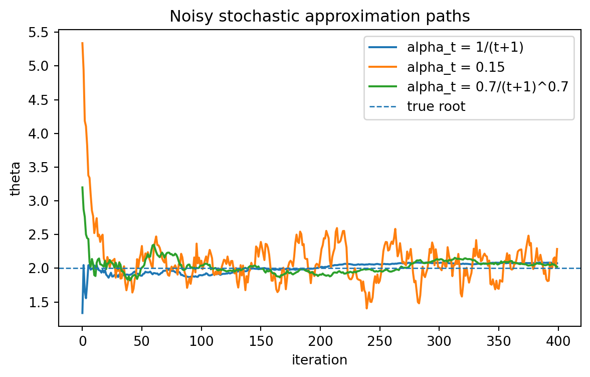
A stochastic approximation update moves toward the root of \(h(\theta)=0\) using noisy observations of \(h(\theta)\). Small learning rates reduce noise but move slowly; large learning rates move quickly but may fluctuate.

17.3.2 Example: one-dimensional stable root

Consider

\[ h(\theta)=a-\theta. \]

The unique root is \(\theta^*=a\). A noisy update has the form

\[ \theta_{t+1} = \theta_t+ \alpha_t\left(a-\theta_t+\varepsilon_{t+1}\right), \]

where \(\mathbb E[\varepsilon_{t+1}\mid\mathcal F_t]=0\). Without noise, this is a weighted average moving toward \(a\):

\[ \theta_{t+1} =(1-\alpha_t)\theta_t+ \alpha_t a. \]

With noise, convergence requires learning rates that are large enough to keep learning but small enough to average out noise.

import numpy as np
import matplotlib.pyplot as plt

rng = np.random.default_rng(7243)
T = 400
a = 2.0
sigma = 0.8

def run_sa(alpha_rule):
    theta = 6.0
    path = []
    for t in range(T):
        alpha = alpha_rule(t)
        noise = rng.normal(0.0, sigma)
        theta = theta + alpha * (a - theta + noise)
        path.append(theta)
    return np.array(path)

paths = {
    "alpha_t = 1/(t+1)": run_sa(lambda t: 1.0 / (t + 1)),
    "alpha_t = 0.15": run_sa(lambda t: 0.15),
    "alpha_t = 0.7/(t+1)^0.7": run_sa(lambda t: 0.7 / ((t + 1) ** 0.7)),
}

plt.figure(figsize=(7, 4))
for name, path in paths.items():
    plt.plot(path, label=name)
plt.axhline(a, linestyle="--", linewidth=1, label="true root")
plt.xlabel("iteration")
plt.ylabel("theta")
plt.title("Noisy stochastic approximation paths")
plt.legend()
plt.show()

Robbins-Monro stochastic approximation for a noisy scalar root.

17.4 14.3 Step-size conditions

The classical diminishing step-size conditions are

\[ \sum_{t=0}^{\infty}\alpha_t=\infty, \qquad \sum_{t=0}^{\infty}\alpha_t^2<\infty. \]

The first condition says that learning never stops too early. The second says that the accumulated variance from noise remains controlled.

A common family is

\[ \alpha_t=\frac{c}{(t+1)^p}. \]

For this family,

\[ \sum_{t=0}^{\infty}\alpha_t=\infty \quad \text{if and only if} \quad p\leq 1, \]

while

\[ \sum_{t=0}^{\infty}\alpha_t^2<\infty \quad \text{if and only if} \quad 2p>1. \]

Thus both classical conditions hold when

\[ \frac{1}{2}<p\leq 1. \]

17.4.1 Interactive: Step-size schedules

This figure compares several learning-rate schedules. A good diminishing schedule keeps \(\sum_t \alpha_t\) large while making \(\sum_t \alpha_t^2\) finite.

import pandas as pd
import numpy as np

T = 10000
schedules = {
    "1/(t+1)^0.4": lambda t: 1 / ((t + 1) ** 0.4),
    "1/(t+1)^0.7": lambda t: 1 / ((t + 1) ** 0.7),
    "1/(t+1)": lambda t: 1 / (t + 1),
    "0.05 constant": lambda t: 0.05,
}

rows = []
for name, rule in schedules.items():
    alphas = np.array([rule(t) for t in range(T)])
    rows.append({
        "schedule": name,
        "sum alpha up to T": alphas.sum(),
        "sum alpha^2 up to T": np.square(alphas).sum(),
        "alpha_T": alphas[-1],
    })

pd.DataFrame(rows)

	schedule	sum alpha up to T	sum alpha^2 up to T	alpha_T
0	1/(t+1)^0.4	417.525500	27.110644	0.025119
1	1/(t+1)^0.7	50.052177	3.042751	0.001585
2	1/(t+1)	9.787606	1.644834	0.000100
3	0.05 constant	500.000000	25.000000	0.050000

17.5 14.4 Martingale-difference noise

Let \(\mathcal F_t\) represent the information available at time \(t\). A sequence \(M_{t+1}\) is a martingale-difference sequence if

\[ \mathbb E[M_{t+1}\mid \mathcal F_t]=0. \]

This condition is the stochastic approximation analogue of unbiased sampling. It does not mean that the update has no variance. It means that, conditional on the current information, the noise does not systematically point in the wrong direction.

In TD learning, define the TD sample update for state \(s\) as

\[ Y_{t+1}(s) = \mathbf 1\{S_t=s\} \left[R_{t+1}+\gamma V_t(S_{t+1})-V_t(s)\right]. \]

The conditional expectation of \(Y_{t+1}(s)\) depends on the current value estimate and the policy-induced transition law. The stochastic update is a noisy version of the expected Bellman correction.

Note

In RL, the noise is more subtle than in iid regression because samples are generated by a Markov chain. Conditional mean-zero arguments are usually made with respect to the filtration generated by the trajectory.

17.6 14.5 Mean drift and deterministic dynamics

The stochastic approximation recursion

\[ \theta_{t+1}=\theta_t+ \alpha_t\left[h(\theta_t)+M_{t+1}\right] \]

has a deterministic counterpart:

\[ \theta_{t+1}=\theta_t+ \alpha_t h(\theta_t). \]

When \(\alpha_t\) is small, this deterministic recursion resembles the ordinary differential equation

\[ \dot \theta(t)=h(\theta(t)). \]

The ODE method studies stochastic approximation by comparing the random discrete-time path to the deterministic flow of this differential equation.

17.6.1 Interactive: ODE method intuition

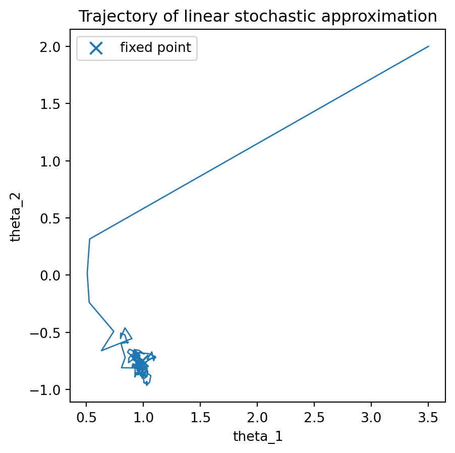
The stochastic recursion fluctuates around the deterministic ODE trajectory. As the step size decreases, the random path increasingly tracks the stable flow toward the equilibrium.

17.6.2 Stable equilibrium

A point \(\theta^*\) is an equilibrium of the ODE if

\[ h(\theta^*)=0. \]

It is locally stable when trajectories starting near \(\theta^*\) move toward it. In one dimension, if \(h\) is differentiable and

\[ h'(\theta^*)<0, \]

then \(\theta^*\) is locally stable. This is the reason that the recursion

\[ \theta_{t+1}=\theta_t+ \alpha_t(a-\theta_t+M_{t+1}) \]

converges toward \(a\): the drift \(h(\theta)=a-\theta\) has derivative \(-1\).

17.7 14.6 Linear stochastic approximation

Many RL algorithms become linear stochastic approximation algorithms after fixing the policy and using linear function approximation. A common form is

\[ \theta_{t+1} = \theta_t+ \alpha_t\left(b-A\theta_t+M_{t+1}\right), \]

where \(A\in\mathbb R^{d\times d}\) and \(b\in\mathbb R^d\).

The mean fixed point satisfies

\[ A\theta^*=b. \]

The associated ODE is

\[ \dot \theta=b-A\theta. \]

The error \(e(t)=\theta(t)-\theta^*\) obeys

\[ \dot e=-Ae. \]

If all eigenvalues of \(A\) have positive real parts, then the deterministic system is stable.

import numpy as np
import matplotlib.pyplot as plt

rng = np.random.default_rng(1401)
A = np.array([[1.2, 0.25], [0.10, 0.8]])
b = np.array([1.0, -0.5])
theta_star = np.linalg.solve(A, b)

T = 500
theta = np.array([3.5, 2.0])
path = [theta.copy()]
for t in range(T):
    alpha = 0.8 / ((t + 1) ** 0.65)
    noise = rng.normal(0.0, 0.4, size=2)
    theta = theta + alpha * (b - A @ theta + noise)
    path.append(theta.copy())
path = np.array(path)

plt.figure(figsize=(5, 5))
plt.plot(path[:, 0], path[:, 1], linewidth=1)
plt.scatter([theta_star[0]], [theta_star[1]], marker="x", s=80, label="fixed point")
plt.xlabel("theta_1")
plt.ylabel("theta_2")
plt.title("Trajectory of linear stochastic approximation")
plt.legend()
plt.axis("equal")
plt.show()

Linear stochastic approximation in two dimensions.

17.8 14.7 Gradient descent as stochastic approximation

Stochastic gradient descent is a special case. Suppose we want to minimize

\[ J(\theta)=\mathbb E[\ell(\theta;Z)]. \]

If \(Z_{t+1}\) is sampled and

\[ G_{t+1}=\nabla_\theta \ell(\theta_t;Z_{t+1}), \]

then

\[ \mathbb E[G_{t+1}\mid \mathcal F_t]=\nabla J(\theta_t). \]

The SGD update is

\[ \theta_{t+1}=\theta_t-\alpha_tG_{t+1}. \]

This has stochastic approximation drift

\[ h(\theta)=-\nabla J(\theta). \]

The associated ODE is gradient flow:

\[ \dot \theta=-\nabla J(\theta). \]

Thus stochastic approximation covers noisy root finding, stochastic fixed-point iteration, and stochastic optimization.

Important

Not every RL update is the gradient of a scalar objective. TD learning is often a stochastic fixed-point method rather than ordinary gradient descent on the mean-squared Bellman error.

17.9 14.8 TD learning as stochastic approximation

Consider a fixed policy \(\pi\) in a finite MDP. The Bellman equation is

\[ V^\pi=T^\pi V^\pi. \]

Equivalently,

\[ h(V)=T^\pi V-V. \]

The deterministic fixed-point iteration is

\[ V_{k+1}=V_k+\alpha_k\left(T^\pi V_k-V_k\right). \]

TD(0) replaces \(T^\pi V_k\) by a one-sample target. If at time \(t\) the chain is in state \(S_t=s\), then

\[ V_{t+1}(s)=V_t(s)+\alpha_t \left[R_{t+1}+\gamma V_t(S_{t+1})-V_t(s)\right]. \]

All other state values are unchanged. The TD error is

\[ \delta_t=R_{t+1}+\gamma V_t(S_{t+1})-V_t(S_t). \]

The update can be written compactly as

\[ V_{t+1}=V_t+\alpha_t\delta_t e_{S_t}, \]

where \(e_{S_t}\) is the coordinate vector for the visited state.

17.9.1 Interactive: TD as stochastic approximation

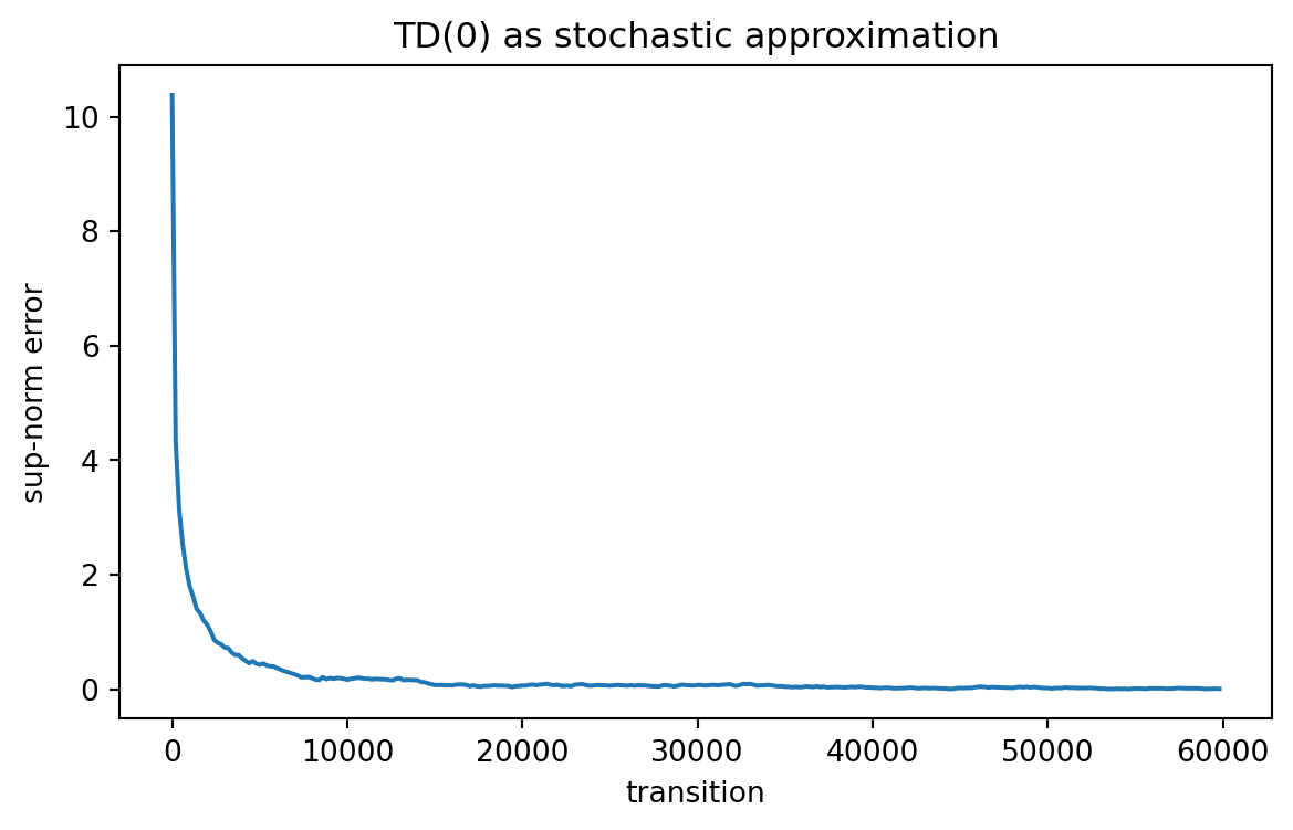
TD learning is a noisy fixed-point method. The expected update moves toward the Bellman fixed point, while sample paths fluctuate around that direction.

import numpy as np
import matplotlib.pyplot as plt

rng = np.random.default_rng(1402)
P = np.array([
    [0.10, 0.80, 0.10],
    [0.20, 0.20, 0.60],
    [0.70, 0.20, 0.10],
])
r = np.array([0.0, 1.0, 2.0])
gamma = 0.90
V_star = np.linalg.solve(np.eye(3) - gamma * P, r)

T = 60000
V = np.zeros(3)
state_visits = np.zeros(3)
s = 0
errors = []
for t in range(T):
    s_next = rng.choice(3, p=P[s])
    reward = r[s] + rng.normal(0.0, 0.25)
    state_visits[s] += 1
    alpha = 0.9 / (state_visits[s] ** 0.65)
    delta = reward + gamma * V[s_next] - V[s]
    V[s] += alpha * delta
    if t % 200 == 0:
        errors.append(np.max(np.abs(V - V_star)))
    s = s_next

plt.figure(figsize=(7, 4))
plt.plot(np.arange(len(errors)) * 200, errors)
plt.xlabel("transition")
plt.ylabel("sup-norm error")
plt.title("TD(0) as stochastic approximation")
plt.show()

print("Exact value:", np.round(V_star, 3))
print("TD estimate:", np.round(V, 3))

TD(0) tracks the exact value function of a fixed policy.

Exact value: [ 8.955 10.02  10.379]
TD estimate: [ 8.958 10.028 10.373]

17.10 14.9 Q-learning as stochastic approximation

Q-learning targets the optimal action-value fixed point

\[ Q^*=T_*Q^*, \]

where

\[ (T_*Q)(s,a)=r(s,a)+\gamma\sum_{s'}P(s'\mid s,a)\max_{a'}Q(s',a'). \]

The tabular Q-learning update is

\[ Q_{t+1}(S_t,A_t) = Q_t(S_t,A_t)+\alpha_t \left[R_{t+1}+\gamma\max_a Q_t(S_{t+1},a)-Q_t(S_t,A_t)\right]. \]

This is a stochastic approximation recursion for the fixed point of the optimal Bellman operator. The mean drift is related to \(T_*Q-Q\), but the update is asynchronous because only one state-action coordinate is changed at a time.

The usual convergence intuition requires:

1. all state-action pairs are visited infinitely often;
2. learning rates for each state-action pair satisfy the classical stochastic approximation conditions;
3. rewards have controlled variance;
4. the finite discounted Bellman optimality operator is a contraction.

Under these conditions, the noise averages out while the mean drift pulls the table toward \(Q^*\).

17.11 14.10 Constant step sizes and tracking

The classical theory often uses diminishing step sizes. In modern reinforcement learning, however, constant step sizes are common:

\[ \alpha_t=\alpha. \]

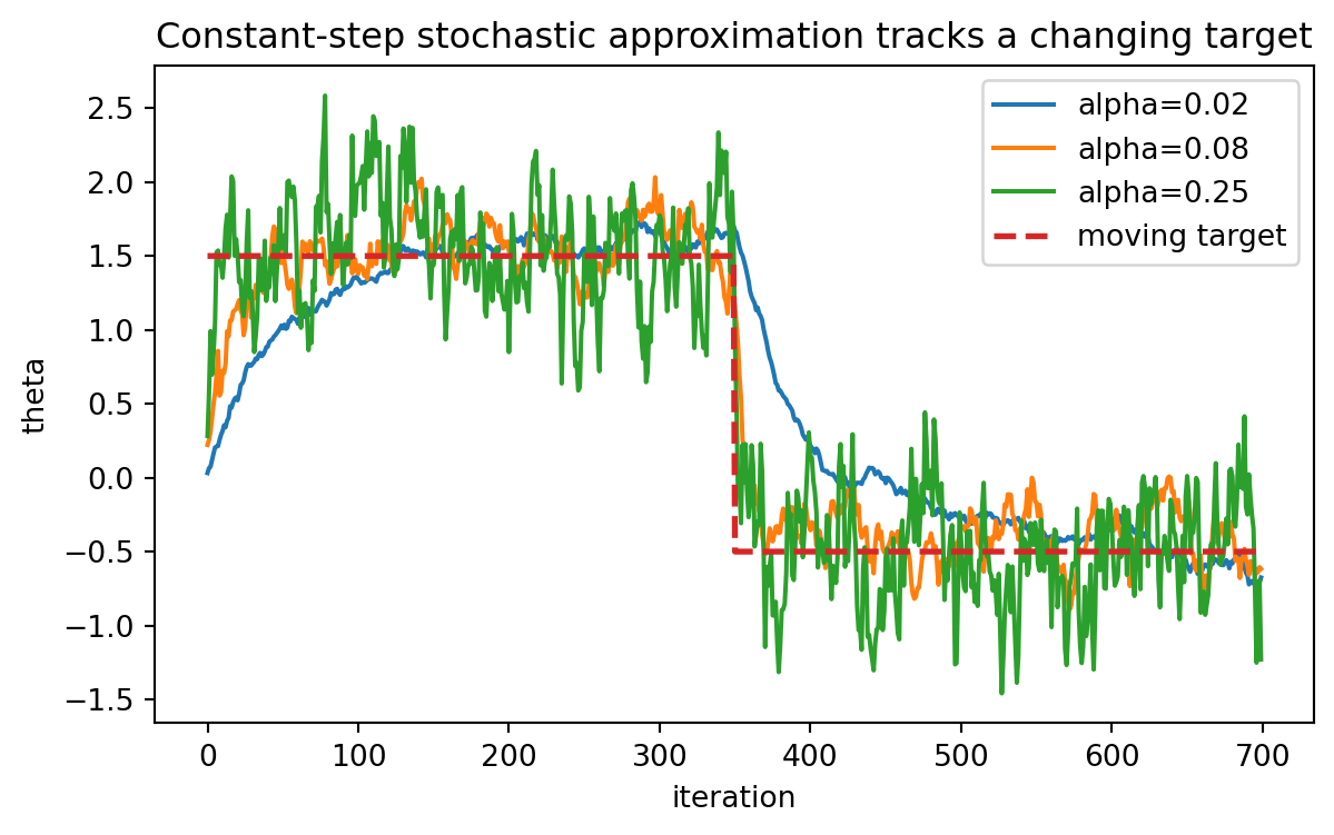
A constant step size does not eliminate noise. Instead, the algorithm tends to fluctuate around the desired solution. This is useful in nonstationary environments, where the target itself may change over time.

There is a tradeoff:

\[ \text{larger } \alpha \quad \Rightarrow \quad \text{faster adaptation but larger steady-state variance}. \]

\[ \text{smaller } \alpha \quad \Rightarrow \quad \text{slower adaptation but smaller steady-state variance}. \]

import numpy as np
import matplotlib.pyplot as plt

rng = np.random.default_rng(1403)
T = 700
sigma = 1.0
alphas = [0.02, 0.08, 0.25]

def target(t):
    return 1.5 if t < 350 else -0.5

plt.figure(figsize=(7, 4))
for alpha in alphas:
    theta = 0.0
    path = []
    for t in range(T):
        a_t = target(t)
        theta += alpha * (a_t - theta + rng.normal(0.0, sigma))
        path.append(theta)
    plt.plot(path, label=f"alpha={alpha}")
plt.plot([target(t) for t in range(T)], linestyle="--", linewidth=2, label="moving target")
plt.xlabel("iteration")
plt.ylabel("theta")
plt.title("Constant-step stochastic approximation tracks a changing target")
plt.legend()
plt.show()

Constant step sizes produce persistent fluctuations around the target.

17.12 14.11 Projection and stability

Stochastic approximation algorithms can diverge if the iterates become unstable. A common theoretical device is projection onto a compact set \(\Theta\):

\[ \theta_{t+1} = \Pi_{\Theta} \left( \theta_t+\alpha_tY_{t+1} \right), \]

where \(\Pi_\Theta\) is Euclidean projection:

\[ \Pi_\Theta(x)=\arg\min_{\theta\in\Theta}\|x-\theta\|_2. \]

Projection is not always used in practical code, but it clarifies theory. It prevents extremely large parameter values and helps make compactness assumptions valid.

In approximate RL, stability is especially important because off-policy learning, bootstrapping, and function approximation may interact badly. This combination is often called the deadly triad.

17.13 14.12 Two-time-scale stochastic approximation

Actor-critic algorithms often update two coupled objects:

\[ \theta_t = \text{actor parameters}, \qquad w_t = \text{critic parameters}. \]

A simplified two-time-scale recursion has the form

\[ w_{t+1}=w_t+\beta_t\left[g(\theta_t,w_t)+N_{t+1}\right], \]

\[ \theta_{t+1}=\theta_t+\alpha_t\left[f(\theta_t,w_t)+M_{t+1}\right]. \]

Usually the critic is updated on the faster time scale:

\[ \frac{\alpha_t}{\beta_t}\to 0. \]

This means that, from the actor’s point of view, the critic approximately equilibrates before the actor changes much. This idea is central in actor-critic theory.

17.13.1 Interactive: Two-time-scale learning

The critic should usually adapt faster than the actor. When the two learning rates are too similar, the actor may chase a poorly estimated critic.

17.14 14.13 AI-assisted stochastic approximation audit

AI tools can be helpful for checking whether an algorithm has been correctly written as a stochastic approximation recursion. The important point is to ask the AI to identify mathematical objects, not merely summarize the algorithm.

17.14.1 AI prompt: identify the stochastic approximation structure

Given an RL update rule, ask an AI assistant:

1. What is the parameter vector \(\theta_t\)?
2. What is the sample update \(Y_{t+1}\)?
3. What is the conditional mean drift \(h(\theta_t)\)?
4. What filtration \(\mathcal F_t\) is natural for this algorithm?
5. What is the martingale-difference noise term?
6. What step-size conditions are required for the classical convergence argument?
7. Is the update a stochastic gradient method, a stochastic fixed-point method, or both?

17.14.2 AI prompt: code-review checklist

Paste a small implementation of TD, SARSA, or Q-learning and ask:

• Are learning rates attached to the correct visited state or state-action pair?
• Does the code accidentally update using the new value where the old value is required?
• Does the behavior policy ensure sufficient exploration?
• Is the target on-policy or off-policy?
• Are random seeds and simulation horizons adequate for a fair comparison?
• Are convergence plots measuring value error, Bellman residual, or return performance?

17.15 14.14 Summary

Stochastic approximation provides the mathematical foundation for many sample-based RL algorithms. The main idea is to study noisy recursions through their conditional mean dynamics.

The key template is

\[ \theta_{t+1} = \theta_t+ \alpha_t\left[h(\theta_t)+M_{t+1}\right]. \]

The term \(h(\theta_t)\) describes the deterministic direction of progress. The term \(M_{t+1}\) describes martingale-difference noise. The step size controls the balance between motion and averaging.

For reinforcement learning, this viewpoint explains why TD learning, SARSA, Q-learning, linear TD, and actor-critic algorithms are not isolated tricks. They are examples of noisy fixed-point or noisy optimization procedures.

17.16 Exercises

17.16.1 Conceptual exercises

1. Explain why stochastic approximation is needed for reinforcement learning but not for exact dynamic programming.
2. In your own words, explain why \(\sum_t\alpha_t=\infty\) and \(\sum_t\alpha_t^2<\infty\) are natural conditions.
3. What is martingale-difference noise? Why is it weaker than assuming iid noise?
4. Explain the ODE method without using measure-theoretic language.
5. Why can constant step sizes be useful in nonstationary environments?

17.16.2 Mathematical exercises

1. Let \(\alpha_t=1/(t+1)^p\). Prove that both classical step-size conditions hold exactly when \(1/2<p\leq 1\).
2. Consider \(\theta_{t+1}=\theta_t+\alpha_t(a-\theta_t)\). Derive an explicit formula for \(\theta_t-a\) in terms of \(\theta_0-a\) and the step sizes.
3. For \(h(\theta)=a-\theta\), show that \(\theta^*=a\) is a globally stable equilibrium of \(\dot\theta=h(\theta)\).
4. For linear stochastic approximation with drift \(b-A\theta\), show that the fixed point is \(\theta^*=A^{-1}b\) when \(A\) is invertible.
5. Write tabular TD(0) as a stochastic approximation recursion and identify the noise term.
6. Write tabular Q-learning as an asynchronous stochastic approximation recursion.
7. Explain why the Bellman contraction is important in the convergence intuition for Q-learning.

17.16.3 Computational exercises

1. Simulate the scalar Robbins-Monro recursion for several values of \(p\) in \(\alpha_t=(t+1)^{-p}\). Compare convergence and variance.
2. Implement TD(0) for a fixed-policy three-state Markov reward process and plot the sup-norm error.
3. Compare constant and diminishing step sizes in TD learning.
4. Simulate a changing target problem and show that constant step sizes track changes better than rapidly diminishing step sizes.
5. Implement a two-time-scale recursion where the critic uses \(\beta_t=(t+1)^{-0.6}\) and the actor uses \(\alpha_t=(t+1)^{-0.9}\).

17.16.4 AI-assisted exercises

1. Ask an AI assistant to rewrite SARSA as stochastic approximation. Check whether it correctly identifies the on-policy target.
2. Ask an AI assistant to compare TD learning and SGD. Find at least one way the comparison can be misleading.
3. Ask an AI assistant to audit a Q-learning implementation for step-size and exploration errors.
4. Ask an AI assistant to explain the ODE method, then rewrite the explanation in your own mathematical language.
5. Ask an AI assistant to generate a convergence plot for stochastic approximation and then verify that the plotted quantity is mathematically meaningful.

17.17 Notes for instructors

For MA Applied Math students, emphasize fixed points, dynamical systems, stability, and ODE intuition. For MS Statistics students, emphasize conditional expectation, martingale-difference noise, stochastic gradients, and sampling variability. This chapter can be taught as the mathematical core connecting TD learning, Q-learning, function approximation, and actor-critic methods.

Recommended references include the original stochastic approximation paper (robbins1951stochastic?), the recursive-algorithm treatment in (kushner2003stochastic?), the ODE-method viewpoint in (borkar2008stochastic?), and the reinforcement learning treatments in (bertsekas1996neuro?), (sutton2018reinforcement?), and (szepesvari2010algorithms?).