Core idea. A fixed policy turns a reinforcement-learning problem into an ordinary Markov chain. Markov chains therefore provide the probability, linear algebra, and asymptotic language behind value functions, policy evaluation, simulation, exploration, and long-run behavior.
5.1 Learning goals
After reading this chapter, students should be able to:
define a finite discrete-time Markov chain using conditional probability;
compute multi-step transition probabilities using matrix powers;
distinguish transient, recurrent, absorbing, irreducible, and aperiodic behavior in finite chains;
find stationary distributions and explain when the chain converges to stationarity;
interpret Markov transition matrices as linear operators on distributions and functions;
use absorbing-chain formulas to compute absorption probabilities and expected absorption times;
connect a Markov chain induced by a fixed policy to reinforcement learning;
estimate a transition matrix from simulated or observed trajectories;
explain how Markov chains appear inside modern AI systems through simulation, state abstraction, and generative modeling.
This chapter is a review, but it is not a superficial review. Reinforcement learning depends on Markov chains at a structural level. Before we optimize a policy, we must understand the stochastic process generated by a policy.
5.2 2.1 Why Markov chains come before reinforcement learning
In supervised learning, a typical observation has the form
\[
(X_i,Y_i), \qquad i=1,\ldots,n,
\]
and the mathematical model often begins with the idea that the observations are independent or conditionally independent. Reinforcement learning is different. The data are generated by interaction over time:
\[
S_0,A_0,R_1,S_1,A_1,R_2,S_2,\ldots .
\]
The next state depends on the current state and current action:
\[
P(S_{t+1}=s' \mid S_t=s,A_t=a).
\]
If a policy \(\pi\) is fixed, then actions are sampled from
\[
\pi(a\mid s)=P(A_t=a\mid S_t=s),
\]
and the state process becomes a Markov chain with transition matrix
This identity is one of the most important bridges in the book. It says that policy evaluation is Markov chain analysis plus rewards. Dynamic programming, temporal-difference learning, and many forms of policy gradient methods all build on this point.
For this chapter, ignore optimization for a moment. Fix the behavior rule and study the stochastic process it creates. Later chapters optimize over such behavior rules.
5.3 2.2 Discrete-time Markov chains
Let \(X_0,X_1,X_2,\ldots\) be random variables taking values in a finite state space
\[
S = \{1,2,\ldots,n\}.
\]
The process is a discrete-time Markov chain if, for every \(t\geq 0\) and every sequence of states with positive conditioning probability,
The initial distribution \(\mu_0\) determines how the chain starts. The transition matrix \(P\) determines how it evolves.
5.3.1 Row-vector convention
In this book, distributions are usually written as row vectors. If
\[
\mu_t(j)=P(X_t=j),
\]
then
\[
\mu_{t+1}=\mu_t P.
\]
Therefore
\[
\mu_t=\mu_0P^t.
\]
Some probability and statistics books use column vectors instead. In that convention, the evolution is \(\mu_{t+1}=P^T\mu_t\). Both conventions are valid. The important thing is to stay consistent.
5.4 2.3 Multi-step transitions and the Chapman-Kolmogorov equations
The entry \((P^t)_{ij}\) gives the probability of moving from state \(i\) to state \(j\) in exactly \(t\) steps:
\[
(P^t)_{ij}=P(X_t=j\mid X_0=i).
\]
This follows from the Chapman-Kolmogorov equations:
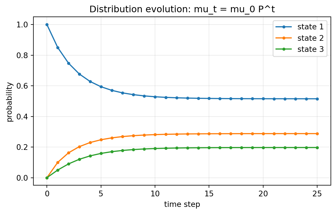
Starting from state \(1\), the initial distribution is
\[
\mu_0=(1,0,0).
\]
The distribution after \(t\) steps is \(\mu_t=\mu_0P^t\).
The plot illustrates a central phenomenon: even though the chain starts at one state, the distribution often moves toward a stable long-run distribution.
5.4.2 Python example: distribution evolution
import numpy as npimport pandas as pdimport matplotlib.pyplot as pltP = np.array([ [0.85, 0.10, 0.05], [0.20, 0.65, 0.15], [0.10, 0.25, 0.65]])mu = np.array([1.0, 0.0, 0.0])T =25history = [mu.copy()]for t inrange(T): mu = mu @ P history.append(mu.copy())history = np.array(history)df = pd.DataFrame(history, columns=["state 1", "state 2", "state 3"])df.head()
This operator viewpoint is essential for reinforcement learning. Bellman equations are equations involving conditional expectations. For example, if a reward \(r(i)\) is received at each state, then the discounted value function satisfies
\[
V(i)=r(i)+\gamma(PV)(i).
\]
Thus
\[
V=r+\gamma PV.
\]
This equation will be studied carefully in Chapter 3.
Distribution side versus function side. The row vector \(\mu\) evolves by \(\mu P\). The value function \(V\) is a column vector and appears in \(PV\). Mixing these two viewpoints is a common source of transposition errors.
5.6 2.5 Communicating classes
A state \(j\) is accessible from state \(i\) if there exists \(t\geq 0\) such that
\[
(P^t)_{ij}>0.
\]
We write \(i\to j\).
States \(i\) and \(j\)communicate if
\[
i\to j \quad \text{and} \quad j\to i.
\]
Communication is an equivalence relation. It partitions the state space into communicating classes.
A Markov chain is irreducible if all states communicate with one another. Equivalently, for every pair \(i,j\), there exists \(t\geq 0\) such that
\[
(P^t)_{ij}>0.
\]
In graph language, create a directed graph with an edge \(i\to j\) whenever \(P_{ij}>0\). The chain is irreducible if this directed graph is strongly connected.
5.6.1 Why irreducibility matters in RL
Irreducibility says that the process can eventually move between all states. In reinforcement learning, this relates to exploration. If a policy never visits part of the state space, then data generated under that policy cannot estimate values or transitions there.
However, irreducibility is not always desirable. In a task with a terminal success state, the chain may intentionally become absorbing after success. The right structure depends on the problem.
5.7 2.6 Periodicity and aperiodicity
The period of a state \(i\) is
\[
d(i)=\gcd\{t\geq 1:(P^t)_{ii}>0\}.
\]
If \(d(i)=1\), the state is aperiodic. If all states in an irreducible chain are aperiodic, the chain is called aperiodic.
is aperiodic because each state has a positive probability of remaining where it is.
Finite-state convergence principle. If a finite Markov chain is irreducible and aperiodic, then it has a unique stationary distribution \(\pi\), and for every initial distribution \(\mu_0\),
This formula is worth remembering. The long-run mass on state \(1\) is proportional to the probability of returning from state \(2\) to state \(1\).
5.8.3 Python example: stationary distribution
The following function computes a stationary distribution by solving a linear system. The equation \(\pi P=\pi\) is singular, so we replace one equation by the normalization condition \(\sum_i\pi_i=1\).
import numpy as npdef stationary_distribution(P):"""Return one stationary distribution of a finite Markov chain. P is assumed to be a row-stochastic matrix. """ P = np.asarray(P, dtype=float) n = P.shape[0] A = P.T - np.eye(n) b = np.zeros(n)# Replace the last equation by sum_i pi_i = 1. A[-1, :] =1.0 b[-1] =1.0return np.linalg.solve(A, b)P = np.array([ [0.85, 0.10, 0.05], [0.20, 0.65, 0.15], [0.10, 0.25, 0.65]])pi = stationary_distribution(P)print(pi)print(pi @ P)
The two printed vectors should agree up to numerical roundoff.
5.9 2.8 Recurrence, transience, and finite chains
Let
\[
T_i^+=\inf\{t\geq 1:X_t=i\}
\]
be the first return time to state \(i\).
State \(i\) is recurrent if
\[
P_i(T_i^+<\infty)=1.
\]
State \(i\) is transient if
\[
P_i(T_i^+<\infty)<1.
\]
For a finite irreducible chain, every state is recurrent. This fact is useful because finite irreducible Markov chains cannot permanently lose probability mass to infinity.
A recurrent state \(i\) is positive recurrent if
\[
E_i[T_i^+]<\infty.
\]
In finite irreducible chains, all states are positive recurrent.
Return-time formula. For a finite irreducible Markov chain with stationary distribution \(\pi\),
\[
E_i[T_i^+]=\frac{1}{\pi_i}.
\]
A state with large stationary probability is visited frequently. A state with small stationary probability has a long expected return time.
In reinforcement learning, this connects to data imbalance. States with small \(\pi_i\) under the behavior policy are rarely observed, so their value estimates may have high variance.
5.10 2.9 Absorbing chains
A state \(i\) is absorbing if
\[
P_{ii}=1.
\]
Once the chain enters an absorbing state, it never leaves. Many episodic reinforcement-learning tasks have absorbing terminal states such as success, failure, or timeout.
Suppose the states are ordered so that transient states come first and absorbing states come last. Then the transition matrix has canonical form
\[
P=
\begin{pmatrix}
Q & R \\
0 & I
\end{pmatrix}.
\]
Here:
\(Q\) describes transitions among transient states;
\(R\) describes transitions from transient states to absorbing states;
\(I\) describes staying in absorbing states.
The fundamental matrix is
\[
N=(I-Q)^{-1}.
\]
The entry \(N_{ij}\) has a probabilistic interpretation:
\[
N_{ij}=E_i\left[\text{number of visits to transient state }j\text{ before absorption}\right].
\]
The matrix of absorption probabilities is
\[
B=NR.
\]
The expected time to absorption from each transient state is
Fundamental matrix N:
          T1        T2        T3
T1  1.395349  1.162791  0.581395
T2  0.232558  1.860465  0.930233
T3  0.058140  0.465116  1.482558

Absorption probabilities B:
    Absorb A  Absorb B
T1  0.476744  0.523256
T2  0.162791  0.837209
T3  0.165698  0.834302

Expected time to absorption:
T1    3.139535
T2    3.023256
T3    2.005814
dtype: float64
5.11 2.10 Reversibility and detailed balance
A Markov chain with stationary distribution \(\pi\) is reversible if
\[
\pi_iP_{ij}=\pi_jP_{ji}
\qquad \text{for all } i,j.
\]
These equations are called detailed balance equations. They say that, in equilibrium, the probability flow from \(i\) to \(j\) equals the probability flow from \(j\) to \(i\).
In the last expression, the index \(j\) is fixed and \(i\) ranges over the second index of row \(j\). Since rows of \(P\) sum to one,
\[
\sum_iP_{ji}=1.
\]
Therefore
\[
(\pi P)_j=\pi_j.
\]
So \(\pi P=\pi\).
Index warning. The expression \(P_{ij}\) means ``from \(i\) to \(j\)’’ in this book. Some references use the transpose convention. When checking detailed balance, always verify the final equation \(\pi P=\pi\).
Reversibility is especially important in Markov chain Monte Carlo. Although MCMC is not the main topic of this book, it gives useful intuition: one can design a transition rule so that the long-run distribution is a desired target distribution.
5.12 2.11 Mixing, eigenvalues, and spectral gaps
For an irreducible aperiodic finite chain, \(\mu_0P^t\to\pi\). A natural quantitative question is: how fast?
One way to measure distance between distributions is total variation distance:
then components associated with \(|\lambda_k|<1\) decay approximately like
\[
|\lambda_k|^t.
\]
The largest nontrivial magnitude
\[
\lambda_* = \max_{k\geq 2}|\lambda_k|
\]
controls the slowest asymptotic mode. The quantity
\[
1-\lambda_*
\]
is called a spectral gap in many settings. A larger gap generally means faster convergence.
This idea reappears later in policy evaluation. The Bellman operator for discounted problems contracts by a factor \(\gamma\), so a large \(\gamma\) creates slow convergence in much the same way that a large \(|\lambda_2|\) slows Markov-chain mixing.
5.13 2.12 Occupancy measures and discounted visitation
Let a fixed policy \(\pi\) induce a transition matrix \(P_{\pi}\). Suppose the initial state distribution is \(\mu_0\). The distribution at time \(t\) is
This distribution tells us which states are emphasized by a discounted reinforcement-learning objective. As \(\gamma\) approaches \(1\), the process cares more about later times. Under suitable ergodicity assumptions, \(d_{\pi,\gamma}\) approaches the stationary distribution of \(P_{\pi}\).
If \(N_i=0\), then the data contain no transitions out of state \(i\). This is a statistical warning: the corresponding row cannot be estimated from the trajectory.
5.14.1 Smoothing
A simple Bayesian or regularized estimate uses pseudocounts:
This is equivalent to using a symmetric Dirichlet prior on each row. The larger \(\alpha\) is, the more the estimate is pulled toward the uniform distribution.
5.14.2 Python example: estimating a transition matrix
5.16 2.15 AI component: Markov state abstractions and generative simulation
Modern AI systems often interact with environments whose true state is high-dimensional. Examples include:
a robot observing images and joint angles;
an autonomous system observing sensor streams;
a language model interacting with a user over a long conversation;
a recommendation system observing user histories;
a scientific AI system choosing experiments adaptively.
In such systems, the raw observation may not be Markov. A useful state representation should summarize the past well enough that the future is predictable from the present. Mathematically, a representation map
\[
z_t=\phi(H_t)
\]
turns a history
\[
H_t=(O_0,A_0,O_1,A_1,\ldots,O_t)
\]
into a state-like variable \(z_t\). The hope is that
If the equality is not plausible, identify which historical variables are missing.
AI caution. Language models are good at generating candidate state variables, but they may ignore hidden confounding, delayed effects, censoring, and nonstationarity. Always translate AI suggestions into explicit conditional probability statements.
5.16.2 Generative simulation perspective
A transition matrix is a simple generative model. Given the current state \(i\), the model samples the next state according to the categorical distribution
In modern AI, a learned world model plays a similar role, but with a much larger state space:
\[
\widehat P_{\theta}(s'\mid s,a).
\]
Planning with a learned transition model is sometimes called model-based reinforcement learning. The finite Markov-chain theory in this chapter is the clean mathematical prototype.
5.17 2.16 Common mistakes
5.17.1 Mistake 1: Confusing \(P_{ij}\) with \(P_{ji}\)
The convention here is
\[
P_{ij}=P(X_{t+1}=j\mid X_t=i).
\]
Rows represent current states. Columns represent next states.
5.17.2 Mistake 2: Assuming \(P^t\) converges for every chain
If the chain is periodic, \(P^t\) may not converge. Irreducibility alone is not enough. Aperiodicity is also needed.
5.17.3 Mistake 3: Estimating transitions for unvisited states
If a trajectory never visits state \(i\), there is no empirical information about row \(i\) of \(P\). This becomes a major issue in offline reinforcement learning.
5.17.4 Mistake 4: Treating one trajectory as independent data
The sequence \(X_0,X_1,\ldots,X_T\) is dependent. Standard independent-sample intuition must be modified.
5.17.5 Mistake 5: Forgetting that a policy changes the chain
Different policies induce different matrices \(P_{\pi}\). A value function is always attached to the dynamics generated by a particular policy.
5.18 2.17 Summary
A finite Markov chain is specified by an initial distribution and a row-stochastic transition matrix. The distribution evolves by
\[
\mu_t=\mu_0P^t.
\]
The same matrix acts on functions by conditional expectation:
\[
(Pf)(i)=E[f(X_{t+1})\mid X_t=i].
\]
Stationary distributions satisfy
\[
\pi=\pi P.
\]
If the finite chain is irreducible and aperiodic, then the distribution converges to the unique stationary distribution. Absorbing chains have a special block form, and the fundamental matrix
\[
N=(I-Q)^{-1}
\]
computes expected visits, absorption probabilities, and expected absorption times.
Estimate the stationary distribution from a long trajectory and compare it to the solution of \(\pi=\pi P\).
Estimate a transition matrix from simulated data for several trajectory lengths \(T\). Plot the Frobenius norm error
\[
\|\widehat P-P\|_F
\]
as a function of \(T\).
Choose two different policies in a small MDP and compute the two induced transition matrices \(P_{\pi_1}\) and \(P_{\pi_2}\). Compare their stationary distributions.
Construct a periodic Markov chain and show numerically that \(\mu_t\) oscillates. Then add a small self-loop probability and show that the modified chain converges.
Build an absorbing random walk on the states \(\{0,1,2,3,4\}\), where \(0\) and \(4\) are absorbing. Compute the probability of absorption at \(4\) starting from each transient state.
5.19.4 AI-assisted exercises
Ask an AI assistant to propose a state representation for an adaptive tutoring system. Translate the proposal into a conditional probability statement and critique whether it is plausibly Markov.
Ask an AI assistant to generate a transition matrix for a three-state learning model with states confused,''developing,’’ and ``mastered.’’ Check whether the matrix is row-stochastic, irreducible, and aperiodic.
Ask an AI assistant to explain the difference between a stationary distribution and a limiting distribution. Verify the explanation using the two-state periodic chain.
5.20 Notes for instructors
For MA Applied Math students, emphasize matrix powers, invariant subspaces, eigenvalues, fixed points, and resolvent identities. For MS Statistics students, emphasize conditional probability, empirical transition estimation, dependence in trajectories, stationary distributions as long-run frequencies, and uncertainty caused by rare states.
A good 75-minute lecture structure is:
Markov property and transition matrix: 15 minutes;
distribution evolution and conditional expectation operator: 15 minutes;
stationary distributions and convergence: 20 minutes;
absorbing chains and fundamental matrix: 15 minutes;
connection to fixed policies in RL: 10 minutes.
For a computational recitation, focus on estimating \(P\) from one simulated trajectory and comparing empirical frequencies to stationary probabilities.
5.21 References
Classical Markov-chain material can be found in standard probability texts. For the reinforcement-learning connection, see (sutton2018reinforcement?), (puterman1994markov?), (bertsekas2012dynamic?), and (szepesvari2010algorithms?). The role of policy-induced Markov chains becomes central in the Markov reward process and Markov decision process chapters that follow.