6  Markov Reward Processes

Core idea. A Markov reward process is a Markov chain with numerical rewards attached to states or transitions. It is the mathematical model for policy evaluation: once a policy is fixed, the agent no longer chooses actions, and the reinforcement learning problem becomes the problem of evaluating a stochastic dynamical system.

The central equation is

\[ V = r + \gamma P V, \]

so that, in a finite discounted problem,

\[ V=(I-\gamma P)^{-1}r. \]

6.1 Learning goals

After reading this chapter, students should be able to:

1. define a finite Markov reward process precisely;
2. distinguish reward random variables, expected rewards, returns, and value functions;
3. derive the Bellman expectation equation by conditioning on the next state;
4. solve a small discounted value problem using linear algebra;
5. interpret value as a discounted occupancy-weighted sum of future rewards;
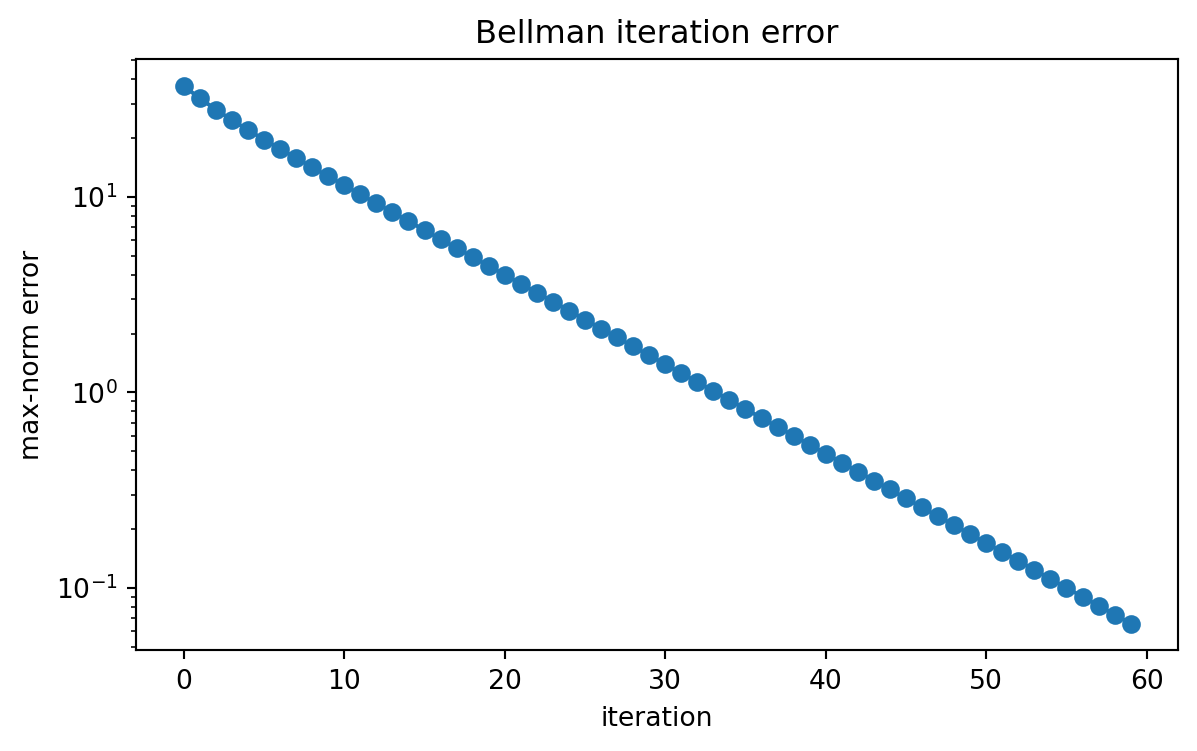
6. prove uniqueness of the discounted value function using contraction mappings;
7. estimate rewards and transition probabilities from sample trajectories;
8. use Python and Plotly.js to visualize value functions, discounting, and simulation uncertainty;
9. use AI tools responsibly to check derivations, debug code, and design small Markov reward models.

6.2 3.1 From Markov chains to reward processes

Chapter sec-ch02-markov-chains-review studied a Markov chain

\[ S_0,S_1,S_2,\ldots \]

with transition probabilities

\[ P(s,s')=P(S_{t+1}=s'\mid S_t=s). \]

A Markov chain describes where the system goes. A Markov reward process also describes what the system earns along the way.

A finite Markov reward process, or MRP, consists of

\[ (\mathcal S,P,r,\gamma), \]

where:

Object	Meaning
\(\mathcal S=\{1,\ldots,m\}\)	finite state space
\(P\in\mathbb R^{m\times m}\)	transition matrix, \(P(s,s')\ge 0\) and \(\sum_{s'}P(s,s')=1\)
\(r\in\mathbb R^m\)	expected one-step reward vector
\(\gamma\in[0,1)\)	discount factor

The expected reward vector is commonly written as

\[ r(s)=\mathbb E[R_{t+1}\mid S_t=s]. \]

In some models the reward may depend on both the current and next state:

\[ r(s,s')=\mathbb E[R_{t+1}\mid S_t=s,S_{t+1}=s']. \]

Then the state-based expected reward is

\[ r(s)=\sum_{s'\in\mathcal S}P(s,s')r(s,s'). \]

Both descriptions are useful. The transition-based version is often closer to modeling, while the state-based version is cleaner for linear algebra.

Why MRPs matter in RL. A policy \(\pi\) in an MDP induces a Markov reward process. Therefore, before optimizing a policy, we must understand how to evaluate a fixed policy. Chapters 4–8 build on this idea.

6.3 3.2 Running example: three-state study model

Consider a simplified student-learning model with three states:

\[ \mathcal S=\{\text{Review},\text{Practice},\text{Mastery}\}. \]

The transition matrix is

\[ P= \begin{pmatrix} 0.55 & 0.40 & 0.05\\ 0.15 & 0.55 & 0.30\\ 0.05 & 0.10 & 0.85 \end{pmatrix}. \]

The reward vector is

\[ r= \begin{pmatrix} -1\\ 2\\ 5 \end{pmatrix}. \]

The interpretation is:

• Review has small negative reward because it costs time and may feel repetitive.
• Practice has positive reward because it builds skill.
• Mastery has high reward because the student can solve problems efficiently.

This example is deliberately small. It lets us see the main mathematics without hiding the structure inside code.

The interactive diagram above represents the transition matrix as a weighted directed graph. Thicker edges correspond to larger transition probabilities. In later chapters, such a graph will arise after a policy is fixed.

6.4 3.3 Return and value

Starting from time \(t\), the discounted return is

\[ G_t = \sum_{k=0}^{\infty}\gamma^kR_{t+k+1} = R_{t+1}+\gamma R_{t+2}+\gamma^2R_{t+3}+\cdots. \]

The value function of an MRP is the conditional expectation

\[ V(s)=\mathbb E[G_t\mid S_t=s]. \]

Because the process is time-homogeneous, \(V(s)\) does not depend on \(t\).

This is the first major conceptual point of reinforcement learning:

A value function is not an immediate reward. It is the expected cumulative future reward, conditional on the current state.

For example, a state with low immediate reward may have high value if it often leads to excellent future states. Conversely, a state with high immediate reward may have low value if it often leads to poor future states.

6.4.1 Effective planning horizon

The discount factor controls how far into the future the value function sees. The total discounted weight is

\[ \sum_{k=0}^{\infty}\gamma^k=\frac{1}{1-\gamma}. \]

Thus \(1/(1-\gamma)\) is often called an effective horizon. It is not a hard cutoff, but it gives a useful scale.

\(\gamma\)	\(1/(1-\gamma)\)	Interpretation
\(0\)	\(1\)	only immediate reward
\(0.50\)	\(2\)	short-term planning
\(0.90\)	\(10\)	medium-term planning
\(0.99\)	\(100\)	long-term planning

The interactive display shows how the value vector changes as \(\gamma\) changes. Large \(\gamma\) magnifies the role of future transitions and can also magnify numerical conditioning issues.

6.5 3.4 Deriving the Bellman expectation equation

The return satisfies the recursive identity

\[ G_t=R_{t+1}+\gamma G_{t+1}. \]

Condition on \(S_t=s\). Then

\[ V(s) =\mathbb E[G_t\mid S_t=s] =\mathbb E[R_{t+1}+\gamma G_{t+1}\mid S_t=s]. \]

By linearity of expectation,

\[ V(s) =\mathbb E[R_{t+1}\mid S_t=s] +\gamma\mathbb E[G_{t+1}\mid S_t=s]. \]

The first term is \(r(s)\). For the second term, condition on the next state:

\[ \mathbb E[G_{t+1}\mid S_t=s] = \sum_{s'\in\mathcal S} P(S_{t+1}=s'\mid S_t=s) \mathbb E[G_{t+1}\mid S_t=s,S_{t+1}=s']. \]

By the Markov property and time homogeneity,

\[ \mathbb E[G_{t+1}\mid S_{t+1}=s']=V(s'). \]

Therefore

\[ V(s)=r(s)+\gamma\sum_{s'\in\mathcal S}P(s,s')V(s'). \]

This is the Bellman expectation equation for an MRP.

Theorem 3.1: Bellman expectation equation for a finite discounted MRP

Let \((\mathcal S,P,r,\gamma)\) be a finite MRP with \(0\le \gamma<1\) and bounded rewards. Then its value function satisfies

\[ V(s)=r(s)+\gamma\sum_{s'}P(s,s')V(s') \]

for every \(s\in\mathcal S\).

The theorem is short, but it is one of the central mathematical patterns of the entire book. Later algorithms approximate this equation when \(P\) and \(r\) are unknown.

6.6 3.5 Linear algebra form

Write \(V\) and \(r\) as column vectors in \(\mathbb R^m\). The Bellman equation becomes

\[ V=r+\gamma PV. \]

Move the second term to the left:

\[ (I-\gamma P)V=r. \]

If \(I-\gamma P\) is invertible, then

\[ V=(I-\gamma P)^{-1}r. \]

This is the cleanest finite-state formula in reinforcement learning.

6.6.1 Why the inverse exists

Because \(P\) is a stochastic matrix, its spectral radius satisfies

\[ \rho(P)\le 1. \]

Hence

\[ \rho(\gamma P)\le \gamma<1. \]

Therefore \(I-\gamma P\) is invertible and

\[ (I-\gamma P)^{-1} = \sum_{k=0}^{\infty}\gamma^kP^k. \]

This is the Neumann series representation.

Theorem 3.2: existence and uniqueness of discounted value

For a finite MRP with \(0\le\gamma<1\), the Bellman equation

\[ V=r+\gamma PV \]

has a unique solution

\[ V=(I-\gamma P)^{-1}r. \]

Proof. Since \(P\) is stochastic, all eigenvalues \(\lambda\) of \(P\) satisfy \(|\lambda|\le 1\). Therefore every eigenvalue of \(\gamma P\) has absolute value at most \(\gamma<1\). Hence \(1\) is not an eigenvalue of \(\gamma P\), so \(I-\gamma P\) is nonsingular. The unique solution follows by ordinary linear algebra. \(\square\)

6.6.2 Python example: solving the linear system

import numpy as np
import matplotlib.pyplot as plt

states = ["Review", "Practice", "Mastery"]
P = np.array([
    [0.55, 0.40, 0.05],
    [0.15, 0.55, 0.30],
    [0.05, 0.10, 0.85]
])
r = np.array([-1.0, 2.0, 5.0])
gamma = 0.90

I = np.eye(len(states))
V = np.linalg.solve(I - gamma * P, r)

for s, v in zip(states, V):
    print(f"{s:>8s}: {v:8.3f}")

plt.figure(figsize=(7, 4))
plt.bar(states, V)
plt.ylabel("value")
plt.title("Discounted value function, gamma = 0.90")
plt.show()

  Review:   22.530
Practice:   29.759
 Mastery:   36.988

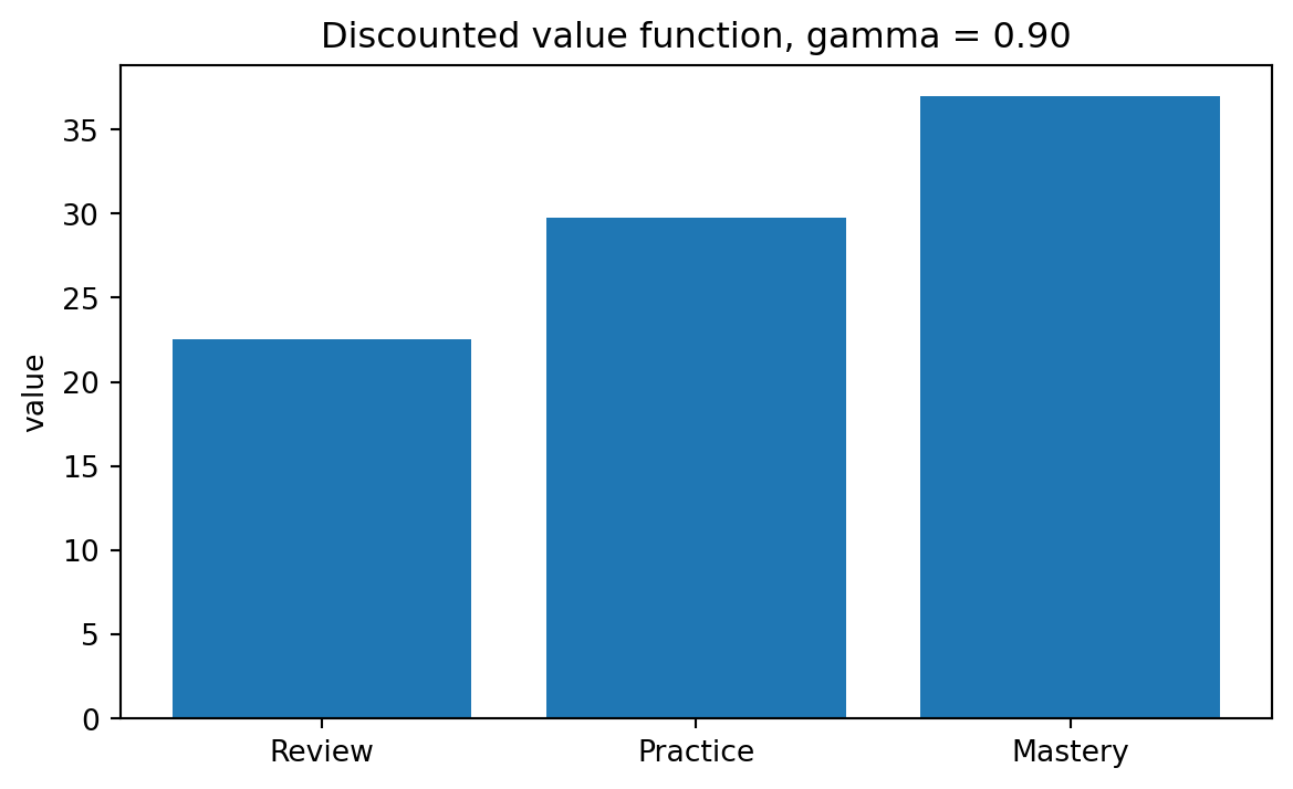
Value function for a three-state Markov reward process.

The values are much larger than the one-step rewards because they include many future rewards. Notice that the value of Review can be positive even though its immediate reward is negative. The reason is that Review can transition into Practice and Mastery.

6.7 3.6 Fixed-point viewpoint

Define the Bellman operator

\[ T:\mathbb R^m\to\mathbb R^m \]

by

\[ (TV)(s)=r(s)+\gamma\sum_{s'}P(s,s')V(s'). \]

In vector form,

\[ TV=r+\gamma PV. \]

The value function is a fixed point:

\[ V=TV. \]

For applied mathematics students, this is a fixed-point problem. For statistics students, it is also a conditional-expectation identity.

6.7.1 Contraction property

Use the max norm

\[ \|V\|_\infty=\max_s |V(s)|. \]

Then

\[ \begin{aligned} \|TV-TW\|_\infty &=\|\gamma P(V-W)\|_\infty\\ &\le \gamma\|V-W\|_\infty. \end{aligned} \]

The inequality follows because each row of \(P\) is a probability vector.

Theorem 3.3: Bellman operator is a contraction

For a finite discounted MRP with \(0\le\gamma<1\),

\[ \|TV-TW\|_\infty\le \gamma\|V-W\|_\infty. \]

Therefore \(T\) has a unique fixed point, and the iteration

\[ V_{k+1}=TV_k \]

converges to \(V\) from any starting vector \(V_0\).

This theorem explains why iterative policy evaluation works. It is not a heuristic. It is a direct consequence of the contraction mapping theorem.

The plot shows how repeated Bellman updates approach the exact solution. The convergence becomes slower when \(\gamma\) is closer to one.

6.7.2 Python example: iterative evaluation

import numpy as np
import matplotlib.pyplot as plt

P = np.array([
    [0.55, 0.40, 0.05],
    [0.15, 0.55, 0.30],
    [0.05, 0.10, 0.85]
])
r = np.array([-1.0, 2.0, 5.0])
gamma = 0.90

V_exact = np.linalg.solve(np.eye(3) - gamma * P, r)
V = np.zeros(3)
errors = []
values = []

for k in range(60):
    values.append(V.copy())
    errors.append(np.max(np.abs(V - V_exact)))
    V = r + gamma * P @ V

plt.figure(figsize=(7, 4))
plt.semilogy(errors, marker="o")
plt.xlabel("iteration")
plt.ylabel("max-norm error")
plt.title("Bellman iteration error")
plt.show()

print("Exact value:", np.round(V_exact, 3))
print("Approximate value after 60 iterations:", np.round(V, 3))

Convergence of Bellman fixed-point iteration.

Exact value: [22.53  29.759 36.988]
Approximate value after 60 iterations: [22.471 29.7   36.929]

6.8 3.7 Discounted occupancy interpretation

The inverse formula has a probabilistic interpretation. From the Neumann series,

\[ V = (I-\gamma P)^{-1}r = \sum_{k=0}^{\infty}\gamma^kP^k r. \]

The \(s\)th component is

\[ V(s) = \sum_{k=0}^{\infty}\gamma^k\sum_{s'}P^k(s,s')r(s'). \]

Here \(P^k(s,s')\) is the probability of being in state \(s'\) after \(k\) steps, starting from \(s\). Thus

\[ V(s) = \sum_{s'} \left(\sum_{k=0}^{\infty}\gamma^kP^k(s,s')\right)r(s'). \]

Define the discounted occupancy weight

\[ D_\gamma(s,s')= \sum_{k=0}^{\infty}\gamma^kP^k(s,s'). \]

Then

\[ V(s)=\sum_{s'}D_\gamma(s,s')r(s'). \]

Matrix-wise,

\[ D_\gamma=(I-\gamma P)^{-1}. \]

The value of a state is a reward-weighted sum of where the Markov chain is expected to spend discounted future time.

The heatmap displays \(D_\gamma\). A large entry \(D_\gamma(s,s')\) means that starting from \(s\), the process expects to spend substantial discounted time in \(s'\).

6.8.1 Normalized discounted state distribution

Sometimes it is useful to multiply by \((1-\gamma)\):

\[ d_\gamma(s,s')=(1-\gamma)D_\gamma(s,s'). \]

For each starting state \(s\),

\[ \sum_{s'}d_\gamma(s,s')=1. \]

So \(d_\gamma(s,\cdot)\) is a probability distribution. If \(T\) is a random time with

\[ P(T=k)=(1-\gamma)\gamma^k, \]

then

\[ d_\gamma(s,s')=P(S_T=s'\mid S_0=s). \]

This gives a clean probabilistic meaning to discounting: choose a random geometrically distributed future time and ask where the chain is then.

6.9 3.8 Reward on transitions

In many applications, rewards depend on transitions rather than only on current states. Suppose

\[ r(s,s')=\mathbb E[R_{t+1}\mid S_t=s,S_{t+1}=s']. \]

Then the Bellman equation is

\[ V(s)=\sum_{s'}P(s,s')\left[r(s,s')+\gamma V(s')\right]. \]

This can be rewritten as the previous formula by defining

\[ r(s)=\sum_{s'}P(s,s')r(s,s'). \]

6.9.1 Example: transition costs

Suppose moving from Review to Practice is rewarding, but falling from Mastery to Review is costly. A transition reward matrix might be

\[ R= \begin{pmatrix} -1 & 2 & 3\\ -2 & 2 & 5\\ -5 & 1 & 5 \end{pmatrix}, \]

where \(R(s,s')\) is the expected reward for moving from \(s\) to \(s'\).

Then the state reward vector is

\[ r(s)=\sum_{s'}P(s,s')R(s,s'). \]

import numpy as np

P = np.array([
    [0.55, 0.40, 0.05],
    [0.15, 0.55, 0.30],
    [0.05, 0.10, 0.85]
])
R = np.array([
    [-1.0, 2.0, 3.0],
    [-2.0, 2.0, 5.0],
    [-5.0, 1.0, 5.0]
])
gamma = 0.90

r_from_transitions = np.sum(P * R, axis=1)
V_transition_reward = np.linalg.solve(np.eye(3) - gamma * P, r_from_transitions)

print("Expected one-step reward from transition rewards:")
print(np.round(r_from_transitions, 3))
print("Value function:")
print(np.round(V_transition_reward, 3))

Expected one-step reward from transition rewards:
[0.4 2.3 4.1]
Value function:
[24.207 28.711 33.078]

6.10 3.9 Simulation viewpoint

The linear system gives the exact value when \(P\) and \(r\) are known. In many reinforcement learning problems, however, the transition matrix and rewards are not known. We observe sample trajectories:

\[ S_0,R_1,S_1,R_2,S_2,\ldots. \]

For a fixed starting state \(s\), one can estimate \(V(s)\) by averaging simulated returns:

\[ \widehat V_N(s) = \frac{1}{N}\sum_{i=1}^N G^{(i)}(s), \]

where each \(G^{(i)}(s)\) is an independent return generated from \(S_0=s\).

This is a Monte Carlo estimator. Under standard assumptions,

\[ \widehat V_N(s)\to V(s) \]

as \(N\to\infty\).

The histogram shows simulated returns from one starting state. The distribution can be wide even when the expected value is well defined. This distinction between a random return and its expectation is essential for statistical thinking in RL.

6.10.1 Python example: Monte Carlo value estimation

import numpy as np
import matplotlib.pyplot as plt

rng = np.random.default_rng(7243)
states = ["Review", "Practice", "Mastery"]
P = np.array([
    [0.55, 0.40, 0.05],
    [0.15, 0.55, 0.30],
    [0.05, 0.10, 0.85]
])
r_mean = np.array([-1.0, 2.0, 5.0])
gamma = 0.90

V_exact = np.linalg.solve(np.eye(3) - gamma * P, r_mean)

def simulate_return(start_state, horizon=200, reward_sd=1.0):
    s = start_state
    G = 0.0
    weight = 1.0
    for t in range(horizon):
        reward = rng.normal(r_mean[s], reward_sd)
        G += weight * reward
        s = rng.choice(len(states), p=P[s])
        weight *= gamma
    return G

N = 1000
start = 0
returns = np.array([simulate_return(start) for _ in range(N)])
running_mean = np.cumsum(returns) / np.arange(1, N + 1)

plt.figure(figsize=(7, 4))
plt.plot(running_mean, label="Monte Carlo running mean")
plt.axhline(V_exact[start], linestyle="--", label="exact value")
plt.xlabel("number of simulated episodes")
plt.ylabel("estimated value")
plt.title("Monte Carlo estimation from Review")
plt.legend()
plt.show()

print("Monte Carlo estimate:", running_mean[-1])
print("Exact value:", V_exact[start])

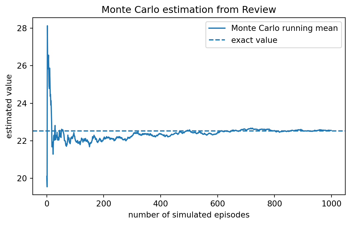
Monte Carlo estimates of value from simulated returns.

Monte Carlo estimate: 22.551141938248207
Exact value: 22.53012048192774

The Monte Carlo estimate converges, but not monotonically. It is an estimator, not a fixed-point iteration. Later chapters compare Monte Carlo, temporal-difference learning, and dynamic programming.

6.11 3.10 Estimating an MRP from data

Suppose we observe a trajectory

\[ (S_0,R_1,S_1,R_2,\ldots,S_T). \]

For finite states, the transition probability can be estimated by empirical frequencies:

\[ \widehat P(s,s') = \frac{N(s,s')}{N(s)}, \]

where

\[ N(s,s')=\sum_{t=0}^{T-1}\mathbf 1\{S_t=s,S_{t+1}=s'\}, \]

and

\[ N(s)=\sum_{s'}N(s,s'). \]

The state reward can be estimated by

\[ \widehat r(s) = \frac{1}{N(s)}\sum_{t:S_t=s}R_{t+1}. \]

Then a plug-in estimate of the value function is

\[ \widehat V=(I-\gamma\widehat P)^{-1}\widehat r. \]

This is simple and mathematically transparent, but it has limitations:

1. rarely visited states have noisy estimates;
2. unvisited states create division-by-zero issues;
3. small transition errors can be amplified when \(\gamma\) is close to one;
4. long-run dependence means the samples are not iid.

import numpy as np

rng = np.random.default_rng(5110)
P_true = np.array([
    [0.55, 0.40, 0.05],
    [0.15, 0.55, 0.30],
    [0.05, 0.10, 0.85]
])
r_true = np.array([-1.0, 2.0, 5.0])
gamma = 0.90

T = 5000
m = 3
states_path = np.zeros(T + 1, dtype=int)
rewards = np.zeros(T)
states_path[0] = 0

for t in range(T):
    s = states_path[t]
    rewards[t] = rng.normal(r_true[s], 1.0)
    states_path[t + 1] = rng.choice(m, p=P_true[s])

counts = np.zeros((m, m))
reward_sums = np.zeros(m)
state_counts = np.zeros(m)

for t in range(T):
    s = states_path[t]
    sp = states_path[t + 1]
    counts[s, sp] += 1
    reward_sums[s] += rewards[t]
    state_counts[s] += 1

P_hat = counts / counts.sum(axis=1, keepdims=True)
r_hat = reward_sums / state_counts
V_hat = np.linalg.solve(np.eye(m) - gamma * P_hat, r_hat)
V_true = np.linalg.solve(np.eye(m) - gamma * P_true, r_true)

print("Estimated P:")
print(np.round(P_hat, 3))
print("Estimated r:", np.round(r_hat, 3))
print("Estimated V:", np.round(V_hat, 3))
print("True V:", np.round(V_true, 3))

Estimated P:
[[0.545 0.413 0.043]
 [0.149 0.548 0.303]
 [0.049 0.101 0.85 ]]
Estimated r: [-1.056  1.993  4.987]
Estimated V: [22.37  29.729 36.936]
True V: [22.53  29.759 36.988]

For MS Statistics students, this section is a bridge to estimation theory. The MRP parameters are estimated from dependent data, then passed through a nonlinear map

\[ (P,r)\mapsto (I-\gamma P)^{-1}r. \]

One may study bias, variance, confidence intervals, concentration bounds, and asymptotic normality for such estimators.

6.12 3.11 Absorbing reward processes

Some Markov reward processes have absorbing terminal states. Suppose the transition matrix has block form

\[ P= \begin{pmatrix} Q & B\\ 0 & I \end{pmatrix}, \]

where \(Q\) describes transitions among transient states and \(I\) describes absorbing states.

In an undiscounted absorbing problem, if absorption occurs with probability one and rewards are accumulated before absorption, the transient value vector satisfies

\[ V_T=r_T+QV_T. \]

Thus

\[ V_T=(I-Q)^{-1}r_T. \]

This is the undiscounted analogue of the discounted formula. The matrix

\[ N=(I-Q)^{-1} \]

is the fundamental matrix of the absorbing chain. The entry \(N(i,j)\) is the expected number of visits to transient state \(j\) starting from transient state \(i\).

Discounted MRPs and absorbing MRPs both reduce value to expected occupancy. The difference is whether future visits are geometrically discounted or stopped by absorption.

6.13 3.12 Connection to policy evaluation

A Markov decision process includes actions. Suppose a policy \(\pi(a\mid s)\) is fixed. Then the policy induces the transition matrix

\[ P_\pi(s,s') = \sum_a\pi(a\mid s)P(s'\mid s,a), \]

and expected reward

\[ r_\pi(s) = \sum_a\pi(a\mid s)r(s,a), \]

or, if rewards also depend on \(s'\),

\[ r_\pi(s) = \sum_a\pi(a\mid s)\sum_{s'}P(s'\mid s,a)r(s,a,s'). \]

The policy value function satisfies

\[ V^\pi=r_\pi+\gamma P_\pi V^\pi. \]

Therefore

\[ V^\pi=(I-\gamma P_\pi)^{-1}r_\pi. \]

This is why MRPs are not optional background. They are the mathematical core of policy evaluation.

6.14 3.13 AI-assisted learning components

AI tools can be useful in this chapter, but they should be used to support mathematical reasoning, not replace it.

6.14.1 Component A: checking a Bellman derivation

Ask an AI assistant:

I have a finite Markov reward process with transition matrix \(P\), reward vector \(r\), and discount factor \(\gamma\). Derive the Bellman equation carefully from the definition \(V(s)=\mathbb E[G_t\mid S_t=s]\). Explicitly state where the Markov property is used.

Then check whether the response includes:

1. the return recursion \(G_t=R_{t+1}+\gamma G_{t+1}\);
2. conditioning on \(S_{t+1}\);
3. the transition probabilities \(P(s,s')\);
4. the final equation \(V=r+\gamma PV\).

If any step is missing, the derivation is incomplete.

6.14.2 Component B: generating a small MRP

Ask an AI assistant to create a three-state or four-state MRP for a real setting, such as studying, inventory, queueing, or exercise habits. Then verify mathematically:

• each row of \(P\) sums to one;
• all entries of \(P\) are nonnegative;
• rewards have a clear interpretation;
• the chosen \(\gamma\) is reasonable;
• the computed value satisfies the Bellman equation numerically.

6.14.3 Component C: debugging value code

A common bug is to write

\[ V=(I-\gamma P^T)^{-1}r \]

instead of

\[ V=(I-\gamma P)^{-1}r. \]

This error depends on whether distributions are represented as row vectors or column vectors. In this book, value vectors are column vectors and \(P(s,s')\) has current state in the row and next state in the column. Therefore the correct formula is

\[ V=r+\gamma PV. \]

When using AI to debug code, always state your convention.

AI caution. Large language models often give correct Bellman formulas but may mix row-vector and column-vector conventions. Always check dimensions. If \(V\) and \(r\) are column vectors, then \(PV\) is valid. If \(\mu\) is a row distribution, then \(\mu P\) is valid.

6.15 3.14 Chapter summary

A Markov reward process is the simplest setting in which the central value equation of reinforcement learning appears. The main ideas are:

• A Markov chain describes state dynamics; an MRP adds rewards.
• The return is a discounted random sum of future rewards.
• The value function is the conditional expectation of return.
• The Bellman equation is obtained by conditioning on the next state.
• In a finite discounted MRP,

\[ V=(I-\gamma P)^{-1}r. \]

• The Bellman operator is a contraction in the max norm.
• Value can be interpreted as discounted future occupancy times rewards.
• Exact evaluation uses linear algebra; sample-based evaluation uses statistical estimation.
• A fixed policy in an MDP induces an MRP.

6.16 3.15 Conceptual exercises

1. Explain in words why a state with negative immediate reward can have positive value.
2. What is the difference between \(R_{t+1}\), \(r(s)\), \(G_t\), and \(V(s)\)?
3. Why does the discount factor \(\gamma<1\) make the infinite-horizon problem mathematically easier?
4. In what sense is a value function a conditional expectation?
5. Why is a Markov reward process the correct model for evaluating a fixed policy?

6.17 3.16 Mathematical exercises

1. Derive the Bellman equation

   \[ V(s)=r(s)+\gamma\sum_{s'}P(s,s')V(s') \]

   using the law of total expectation.

2. Prove that if \(P\) is stochastic, then

   \[ \|Px\|_\infty\le \|x\|_\infty \]

   for every vector \(x\in\mathbb R^m\).

3. Use Exercise 2 to prove that the Bellman operator is a contraction.

4. Prove the Neumann series identity

   \[ (I-\gamma P)^{-1}=\sum_{k=0}^{\infty}\gamma^kP^k. \]

5. Let

   \[ P=\begin{pmatrix} 0.7 & 0.3\\ 0.2 & 0.8 \end{pmatrix}, \qquad r=\begin{pmatrix}1\\4\end{pmatrix}, \qquad \gamma=0.9. \]

   Compute \(V\) exactly by solving a \(2\times 2\) linear system.

6. Suppose rewards depend on transitions. Show that

   \[ V(s)=\sum_{s'}P(s,s')\{r(s,s')+\gamma V(s')\} \]

   can be rewritten as \(V=r+\gamma PV\) by defining an appropriate state reward vector.

7. Let \(D_\gamma=(I-\gamma P)^{-1}\). Prove that each row of \((1-\gamma)D_\gamma\) sums to one.

6.18 3.17 Computational exercises

1. Implement the three-state study MRP from this chapter and compute \(V\) for \(\gamma=0,0.5,0.9,0.99\).
2. Plot the condition number of \(I-\gamma P\) as a function of \(\gamma\in[0,0.99]\).
3. Simulate returns from each starting state and compare Monte Carlo estimates to the exact values.
4. Estimate \(P\) and \(r\) from one long trajectory. Study how the error in \(\widehat V\) changes as \(T\) increases.
5. Modify the transition matrix so that Mastery is absorbing. Compare the value function before and after this change.
6. Build a four-state MRP for a queueing, finance, health, or education example. Explain the meaning of each state and reward.

6.19 3.18 AI-assisted exercises

1. Ask an AI assistant to create a real-world MRP with four states. Then check whether its transition matrix is valid. Correct any invalid rows.
2. Ask an AI assistant to derive the Bellman equation. Identify whether it clearly distinguishes random rewards from expected rewards.
3. Ask an AI assistant to write Python code for value computation. Test the code on a two-state example where you know the answer by hand.
4. Ask an AI assistant to explain the discounted occupancy matrix. Rewrite the explanation in your own mathematical language.
5. Ask an AI assistant to propose a reward function for an education or healthcare problem. Critique whether the reward might create unintended behavior.

6.20 3.19 Notes for instructors

This chapter should be taught slowly because it contains the first complete mathematical mechanism of the book. A useful lecture sequence is:

1. define MRPs as Markov chains plus rewards;
2. derive the Bellman equation from conditional expectation;
3. solve \(V=(I-\gamma P)^{-1}r\) in a small example;
4. interpret the inverse as discounted occupancy;
5. compare exact linear algebra with Monte Carlo simulation;
6. preview policy evaluation by replacing \(P\) with \(P_\pi\) and \(r\) with \(r_\pi\).

For MA Applied Math students, emphasize fixed points, linear systems, spectral radius, and contractions. For MS Statistics students, emphasize conditional expectation, sampling, simulation, plug-in estimation, and uncertainty.

6.21 References

The Bellman expectation equation and Markov reward process viewpoint are standard foundations for dynamic programming and reinforcement learning; see (bellman1957dynamic?), (puterman1994markov?), (bertsekas2012dynamic?), (sutton2018reinforcement?), and (szepesvari2010algorithms?).