---
title: "Chapter 1: The World as Numbers"
subtitle: "How objects become vectors"
format:
html:
toc: true
toc-depth: 3
number-sections: true
code-fold: true
code-tools: true
jupyter: python3
---
## Opening Story: Before a Computer Can Think, It Must Measure
A person looks at a photograph and says, "That is a dog."
A computer does not begin with the word *dog*.
It begins with numbers.
A digital image is a grid of pixel values. A song is a long sequence of sound measurements. A sentence can be turned into word counts or word embeddings. A house listing can be turned into size, location, bedrooms, tax, age, and price. A patient record can be turned into blood pressure, cholesterol, age, lab values, diagnoses, and medication history.
This is one of the central translations of the modern world:
> To compute with the world, we first turn part of the world into numbers.
Linear algebra begins with this translation.
It does not begin with a complicated formula. It begins with a choice:
> What numbers will we use to describe the object?
Once that choice is made, an object becomes a **vector**. A vector is a list of numbers, but in applications it is never merely a list. Each coordinate carries meaning. Each coordinate is a measurement, a feature, a count, a rating, a location, a signal value, or some other piece of information.
This chapter is the doorway into the book. We will not yet do much algebra. Instead, we will learn the first habit of linear algebraic thinking:
> See the world as objects. Choose features. Store the features as vectors. Study the geometry of the resulting data.
## Learning Goals
By the end of this chapter, you should be able to:
1. Explain why real-world objects are often represented by numbers.
2. Define a vector as a structured list of coordinates.
3. Interpret coordinates as meaningful features, not just entries.
4. Translate simple objects into feature vectors.
5. View a data table as a collection of vectors.
6. Plot two-dimensional and three-dimensional data vectors.
7. Explain why high-dimensional data appears naturally in images, text, recommendation systems, and AI.
8. Recognize that every representation captures some information and loses other information.
9. Use Python to create, visualize, compare, and scale simple vectors.
## 1.1 The First Move: Choose Features
Imagine describing a house.
In ordinary language, we may say:
> The house is medium-sized, has three bedrooms, is not too far from the city, and is expensive.
That sentence is useful to a person, but it is not directly useful to a computer. A computer needs a structured representation.
We may instead describe the house by four numbers:
$$
x =
\begin{bmatrix}
1800 \\
3 \\
12 \\
550000
\end{bmatrix}.
$$
This vector means something only after we say what each coordinate represents:
$$
\begin{bmatrix}
\text{square feet} \\
\text{number of bedrooms} \\
\text{distance to city center in miles} \\
\text{price in dollars}
\end{bmatrix}
=
\begin{bmatrix}
1800 \\
3 \\
12 \\
550000
\end{bmatrix}.
$$
The object is the house. The features are the measurements. The vector is the mathematical representation.
::: {.callout-important}
## Main Idea
A vector is a structured list of numbers used to represent an object.
Each coordinate answers a question about the object.
:::
For the house above, the coordinates answer questions such as:
- How large is the house?
- How many bedrooms does it have?
- How far is it from the city center?
- What is its price?
A different project may choose different questions. For example, an architect may care about sunlight and floor plan. A bank may care about price, income, mortgage rate, and risk. A city planner may care about density, tax value, zoning, and transportation.
The vector depends on the purpose.
## 1.2 A Vector Is a Sentence Written in Numbers
A sentence is not just a sequence of words. It has meaning because the words are arranged in a language.
A vector is similar. It is not just a sequence of numbers. It has meaning because the coordinates belong to a chosen feature system.
For example,
$$
p =
\begin{bmatrix}
68 \\
150 \\
20
\end{bmatrix}
$$
could describe a person using the features
$$
\begin{bmatrix}
\text{height in inches} \\
\text{weight in pounds} \\
\text{age in years}
\end{bmatrix}.
$$
But the same numerical vector could also describe something completely different:
$$
\begin{bmatrix}
\text{temperature} \\
\text{humidity} \\
\text{wind speed}
\end{bmatrix}
=
\begin{bmatrix}
68 \\
150 \\
20
\end{bmatrix}.
$$
That second interpretation is probably suspicious because humidity is usually measured as a percentage and $150$ percent humidity does not make sense in ordinary weather reporting. This is a useful lesson: coordinates are not only numbers. They have units, ranges, and context.
::: {.callout-note}
## Representation Is a Language
A vector becomes meaningful only when we know the coordinate language.
Before computing with a vector, ask:
> What does each coordinate mean?
:::
## 1.3 Definition: Object, Feature, Coordinate, Vector
We now make the language more precise.
::: {.callout-important}
## Definition: Feature Vector
An **object** is something we want to describe or study.
A **feature** is a measurable or encoded attribute of the object.
A **feature vector** is an ordered list of feature values:
$$
x =
\begin{bmatrix}
x_1 \\
x_2 \\
\vdots \\
x_n
\end{bmatrix}.
$$
The number $x_i$ is the $i$th **coordinate** or **component** of $x$.
:::
The order matters. The vector
$$
\begin{bmatrix}
1800 \\
3 \\
12 \\
550000
\end{bmatrix}
$$
is not the same representation as
$$
\begin{bmatrix}
550000 \\
12 \\
3 \\
1800
\end{bmatrix},
$$
unless we also change the coordinate dictionary. A coordinate dictionary tells us what each position means.
For the house example, the coordinate dictionary is:
| Coordinate | Meaning | Unit |
|---:|---|---|
| $x_1$ | size | square feet |
| $x_2$ | bedrooms | count |
| $x_3$ | distance to city center | miles |
| $x_4$ | price | dollars |
This table is as important as the vector itself.
## 1.4 A Feature Map: The Function That Turns Objects into Vectors
The process of turning an object into a vector can be viewed as a function.
If $\mathcal{O}$ is a collection of objects, then a feature map has the form
$$
\phi : \mathcal{O} \to \mathbb{R}^n.
$$
Here $\phi$ takes an object and returns a vector with $n$ real-number coordinates.
For example, if $H$ is a house, then
$$
\phi(H)
=
\begin{bmatrix}
\text{size of } H \\
\text{bedrooms in } H \\
\text{distance from } H \text{ to city center} \\
\text{price of } H
\end{bmatrix}.
$$
This notation may look formal, but the idea is simple:
> A feature map is a measurement machine.
It takes something from the world and produces a vector.
::: {.callout-tip}
## Why This Matters
Much of applied linear algebra begins after a feature map has already been chosen.
But in real applications, choosing the feature map is often the most important step.
:::
## 1.5 Data Tables Are Collections of Vectors
A dataset is often stored as a table. Each row represents one object. Each column represents one feature.
Consider four houses:
| House | Size | Bedrooms | Distance | Price |
|---|---:|---:|---:|---:|
| A | 1200 | 2 | 8 | 400000 |
| B | 1800 | 3 | 12 | 550000 |
| C | 2400 | 4 | 20 | 610000 |
| D | 1000 | 2 | 5 | 420000 |
Each row can be viewed as a vector. For example,
$$
x_B =
\begin{bmatrix}
1800 \\
3 \\
12 \\
550000
\end{bmatrix}.
$$
The whole table can be viewed as a stack of vectors:
$$
X =
\begin{bmatrix}
1200 & 2 & 8 & 400000 \\
1800 & 3 & 12 & 550000 \\
2400 & 4 & 20 & 610000 \\
1000 & 2 & 5 & 420000
\end{bmatrix}.
$$
This rectangular array is called a **matrix**. We will study matrices deeply later. For now, think of a matrix as a data table made of vectors.
::: {.callout-note}
## Rows and Columns
In many data science settings:
- rows are objects,
- columns are features,
- each row is a vector,
- the whole table is a matrix.
:::
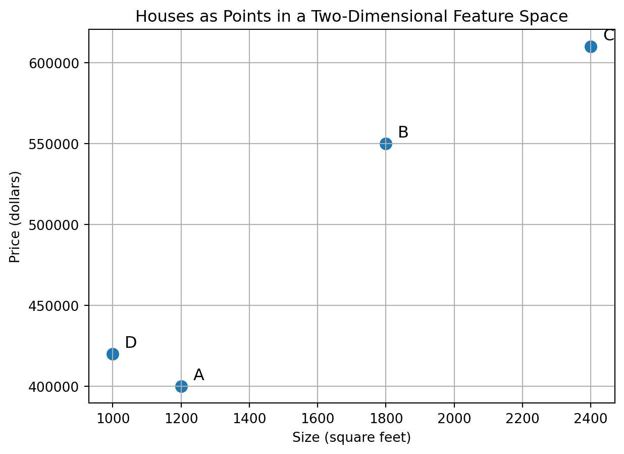
## 1.6 Two Features Create a Plane
When each object has two features, we can draw the objects as points in a plane.
Suppose we represent each house only by size and price:
$$
\begin{bmatrix}
\text{size} \\
\text{price}
\end{bmatrix}.
$$
Then House B becomes
$$
\begin{bmatrix}
1800 \\
550000
\end{bmatrix}.
$$
This is a point in a two-dimensional feature space.
```{python}
import numpy as np
import matplotlib.pyplot as plt

# House data
sizes = np.array([1200, 1800, 2400, 1000])
prices = np.array([400000, 550000, 610000, 420000])
labels = np.array(["A", "B", "C", "D"])

plt.figure(figsize=(7, 5))
plt.scatter(sizes, prices, s=70)

for size, price, label in zip(sizes, prices, labels):
    plt.text(size + 35, price + 4000, label, fontsize=12)

plt.xlabel("Size (square feet)")
plt.ylabel("Price (dollars)")
plt.title("Houses as Points in a Two-Dimensional Feature Space")
plt.grid(True)
plt.show()
```
In ordinary geometry, a point is just a location. In data geometry, a point is an object described by features.
The plane has become a space of houses.
::: {.callout-tip}
## Data Space
A **data space** is a coordinate space whose axes represent features.
When objects become vectors, they become points in data space.
:::
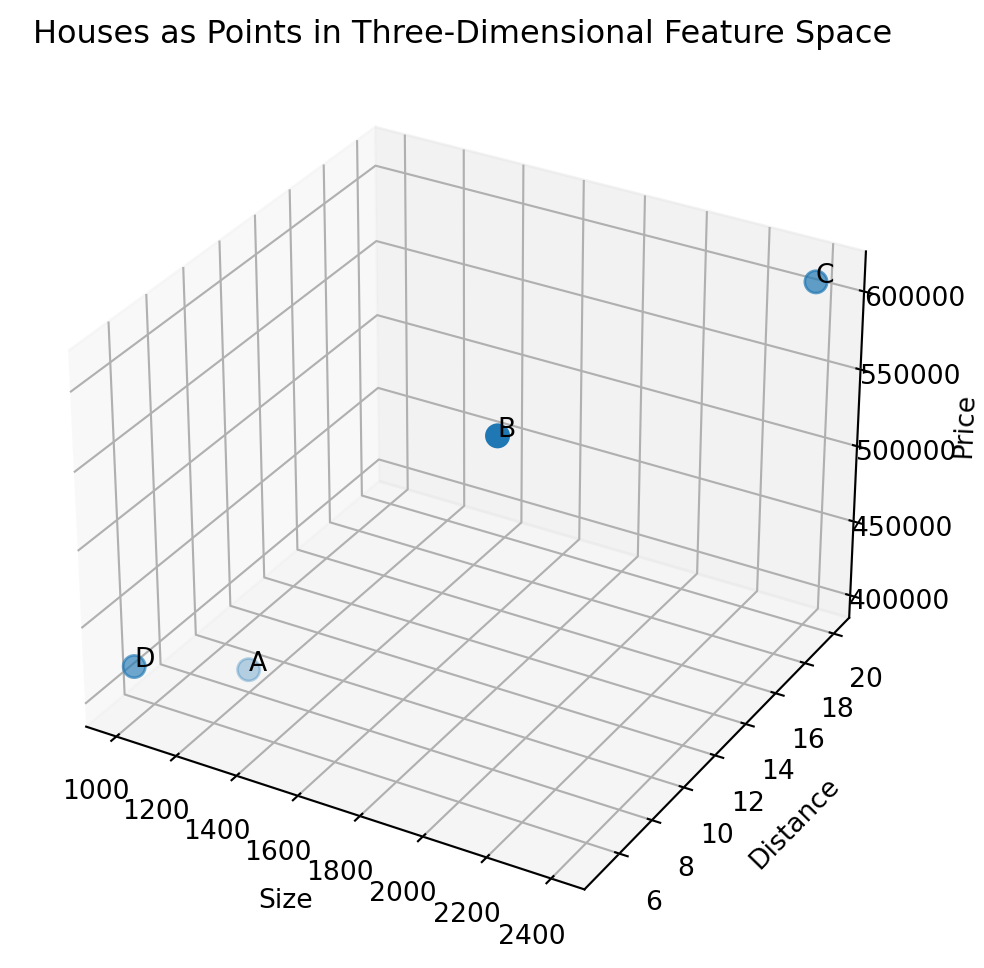
## 1.7 Three Features Create Space
With three features, objects become points in three-dimensional space.
For example, we may represent a house by
$$
\begin{bmatrix}
\text{size} \\
\text{distance} \\
\text{price}
\end{bmatrix}.
$$
```{python}
from mpl_toolkits.mplot3d import Axes3D  # noqa: F401

sizes = np.array([1200, 1800, 2400, 1000])
distances = np.array([8, 12, 20, 5])
prices = np.array([400000, 550000, 610000, 420000])
labels = np.array(["A", "B", "C", "D"])

fig = plt.figure(figsize=(8, 6))
ax = fig.add_subplot(111, projection="3d")

ax.scatter(sizes, distances, prices, s=70)

for size, distance, price, label in zip(sizes, distances, prices, labels):
    ax.text(size, distance, price, label)

ax.set_xlabel("Size")
ax.set_ylabel("Distance")
ax.set_zlabel("Price")
ax.set_title("Houses as Points in Three-Dimensional Feature Space")
plt.show()
```
Three dimensions are still visual. We can rotate the plot in our imagination or with software.
But real data often has far more than three features.
## 1.8 Many Features Create High-Dimensional Space
A house listing may include:
- size,
- bedrooms,
- bathrooms,
- year built,
- lot size,
- school rating,
- distance to downtown,
- distance to public transportation,
- crime rate,
- property tax,
- mortgage rate,
- listing price.
That is already twelve features. The vector would live in $\mathbb{R}^{12}$.
A small grayscale image of size $28 \times 28$ has $784$ pixel values, so it can be treated as a vector in $\mathbb{R}^{784}$.
A color image of size $224 \times 224$ has three color channels, so it contains
$$
224 \times 224 \times 3 = 150528
$$
numbers.
That image can be viewed as a vector in $\mathbb{R}^{150528}$.
We cannot draw $\mathbb{R}^{150528}$. But we can compute in it.
::: {.callout-important}
## High-Dimensional Thinking
Modern data is often high-dimensional.
Linear algebra gives us tools for spaces we cannot draw.
:::
## 1.9 Four Everyday Examples of Vectorization
The act of turning an object into a vector is sometimes called **vectorization**. Here are four examples that will return throughout the book.
### Houses
A house can become a vector of measurements:
$$
x_{\text{house}}=
\begin{bmatrix}
\text{size} \\
\text{bedrooms} \\
\text{bathrooms} \\
\text{distance} \\
\text{price}
\end{bmatrix}.
$$
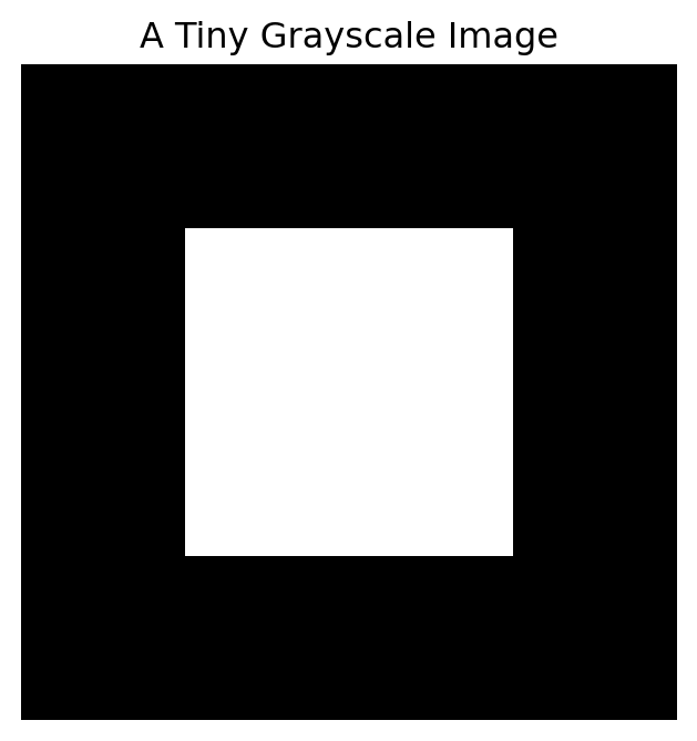
### Images
A grayscale image can become a grid of pixel intensities:
$$
\begin{bmatrix}
0 & 0 & 0 & 0 \\
0 & 255 & 255 & 0 \\
0 & 255 & 255 & 0 \\
0 & 0 & 0 & 0
\end{bmatrix}.
$$
Here $0$ means black, $255$ means white, and values between them represent shades of gray.
```{python}
tiny_image = np.array([
    [0, 0, 0, 0],
    [0, 255, 255, 0],
    [0, 255, 255, 0],
    [0, 0, 0, 0]
])

plt.figure(figsize=(4, 4))
plt.imshow(tiny_image, cmap="gray", vmin=0, vmax=255)
plt.title("A Tiny Grayscale Image")
plt.axis("off")
plt.show()
```
Later, we will use linear algebra to compress, denoise, and transform images.
### Text
A document can become a vector by counting words. Suppose our vocabulary is
$$
[\text{math}, \text{data}, \text{AI}, \text{model}].
$$
The sentence
> AI and data need a model.
can be represented as
$$
\begin{bmatrix}
0 \\
1 \\
1 \\
1
\end{bmatrix},
$$
because it contains the words data, AI, and model, but not math.
Modern AI systems use more advanced vector representations called embeddings, but the first idea is the same:
> Text becomes numbers before a machine can compute with it.
### Movie Preferences
A person can become a vector of ratings. Suppose the coordinates correspond to five movies. Then
$$
a =
\begin{bmatrix}
5 \\
4 \\
1 \\
1 \\
5
\end{bmatrix}
$$
could represent Alice's ratings. Recommendation systems compare such vectors to find users with similar taste or movies with similar audiences.
## 1.10 Similarity Begins After Representation
Once objects become vectors, we can compare them.
Suppose three users rate three movies:
$$
a =
\begin{bmatrix}
5 \\
4 \\
1
\end{bmatrix},
\qquad
b =
\begin{bmatrix}
5 \\
5 \\
2
\end{bmatrix},
\qquad
c =
\begin{bmatrix}
1 \\
1 \\
5
\end{bmatrix}.
$$
Alice and Bob probably have similar taste. Alice and Carol probably have different taste.
One simple way to compare two vectors is to compute the distance between them:
$$
\text{distance}(u,v)=\|u-v\|.
$$
We will study distance carefully later. For now, the formula says:
> Subtract the vectors and measure the size of the difference.
```{python}
alice = np.array([5, 4, 1])
bob = np.array([5, 5, 2])
carol = np.array([1, 1, 5])

distance_alice_bob = np.linalg.norm(alice - bob)
distance_alice_carol = np.linalg.norm(alice - carol)

distance_alice_bob, distance_alice_carol
```
The distance from Alice to Bob is smaller than the distance from Alice to Carol. This agrees with our intuition.
::: {.callout-important}
## Comparison Becomes Geometry
Once objects become vectors, comparing objects becomes a geometric problem.
This is one reason linear algebra is central to data science, machine learning, statistics, signal processing, and AI.
:::
## 1.11 Units Can Change the Geometry
Numbers are not neutral. Their units matter.
Consider the house vector
$$
\begin{bmatrix}
1800 \\
550000
\end{bmatrix},
$$
where the first coordinate is size in square feet and the second coordinate is price in dollars.
The price coordinate is much larger than the size coordinate. If we compute distances directly, price may dominate the comparison.
That does not necessarily mean price is more important. It may only mean that price is measured in large units.
Let us see this in Python.
```{python}
# Two houses represented by [size, price]
house_1 = np.array([1800, 550000])
house_2 = np.array([1900, 575000])
house_3 = np.array([2400, 560000])

np.linalg.norm(house_1 - house_2), np.linalg.norm(house_1 - house_3)
```
House 1 and House 3 have very different sizes, but their prices are relatively close. Because the price coordinate is large, direct distance can make size differences appear less important.
A common fix is to scale each feature.
```{python}
# A small data matrix with columns [size, price]
houses = np.array([
    [1800, 550000],
    [1900, 575000],
    [2400, 560000]
])

# Standardize each column: subtract mean and divide by standard deviation
means = houses.mean(axis=0)
stds = houses.std(axis=0)
houses_scaled = (houses - means) / stds

houses_scaled
```
Now both features are measured on a comparable scale.
```{python}
scaled_distance_12 = np.linalg.norm(houses_scaled[0] - houses_scaled[1])
scaled_distance_13 = np.linalg.norm(houses_scaled[0] - houses_scaled[2])

scaled_distance_12, scaled_distance_13
```
The lesson is not that scaling is always correct. The lesson is that representation choices affect geometry.
::: {.callout-warning}
## Warning: Coordinates Have Units
Changing units can change distances, similarities, clusters, and predictions.
Before comparing vectors, ask:
> Are the coordinates measured on compatible scales?
:::
## 1.12 Categorical Information Also Needs Encoding
Not every feature is naturally numerical.
Suppose a house has a heating type:
- gas,
- electric,
- oil.
A computer cannot directly compute with the word "gas." We need an encoding.
One common method is called **one-hot encoding**:
$$
\text{gas} =
\begin{bmatrix}
1 \\
0 \\
0
\end{bmatrix},
\qquad
\text{electric} =
\begin{bmatrix}
0 \\
1 \\
0
\end{bmatrix},
\qquad
\text{oil} =
\begin{bmatrix}
0 \\
0 \\
1
\end{bmatrix}.
$$
Each category gets its own coordinate.
This is another example of a representation choice. We turned a word into a vector by deciding how the categories should be encoded.
::: {.callout-note}
## Not All Numbers Are Measurements
Some coordinates are measurements, such as height or price.
Other coordinates are encodings, such as one-hot variables for categories.
Both can be used in vectors, but they should be interpreted differently.
:::
## 1.13 What a Representation Captures and What It Loses
Every representation is selective.
A house vector may capture size, bedrooms, distance, and price. It may miss sunlight, street noise, architecture, neighborhood feeling, and whether the house feels like home.
A movie-rating vector may capture numerical preferences. It may miss memories, mood, genre, language, acting style, and why someone loved a movie.
A word-count vector may capture which words appear. It may miss sarcasm, context, word order, tone, and cultural meaning.
A medical vector may capture lab values. It may miss uncertainty, patient experience, access to care, and the story behind the numbers.
This does not make vector representations bad. It makes them tools.
A tool is powerful when we understand what it is designed to do and what it cannot do.
::: {.callout-important}
## Mathematical Humility
A vector is not the object itself.
A vector is a structured shadow of the object.
Linear algebra teaches us how to reason with that shadow.
:::
## 1.14 Mini-Lab: Build a Tiny Dataset
In this mini-lab, we create a small dataset and treat each row as a vector.
```{python}
import pandas as pd

students = pd.DataFrame({
    "student": ["A", "B", "C", "D"],
    "math": [92, 85, 70, 88],
    "writing": [78, 90, 82, 84],
    "science": [95, 80, 75, 91]
})

students
```
The numerical part of this table is a data matrix.
```{python}
X = students[["math", "writing", "science"]].to_numpy()
X
```
Each row is a vector:
```{python}
student_A = X[0]
student_B = X[1]

student_A, student_B
```
We can compare two students by distance:
```{python}
np.linalg.norm(student_A - student_B)
```
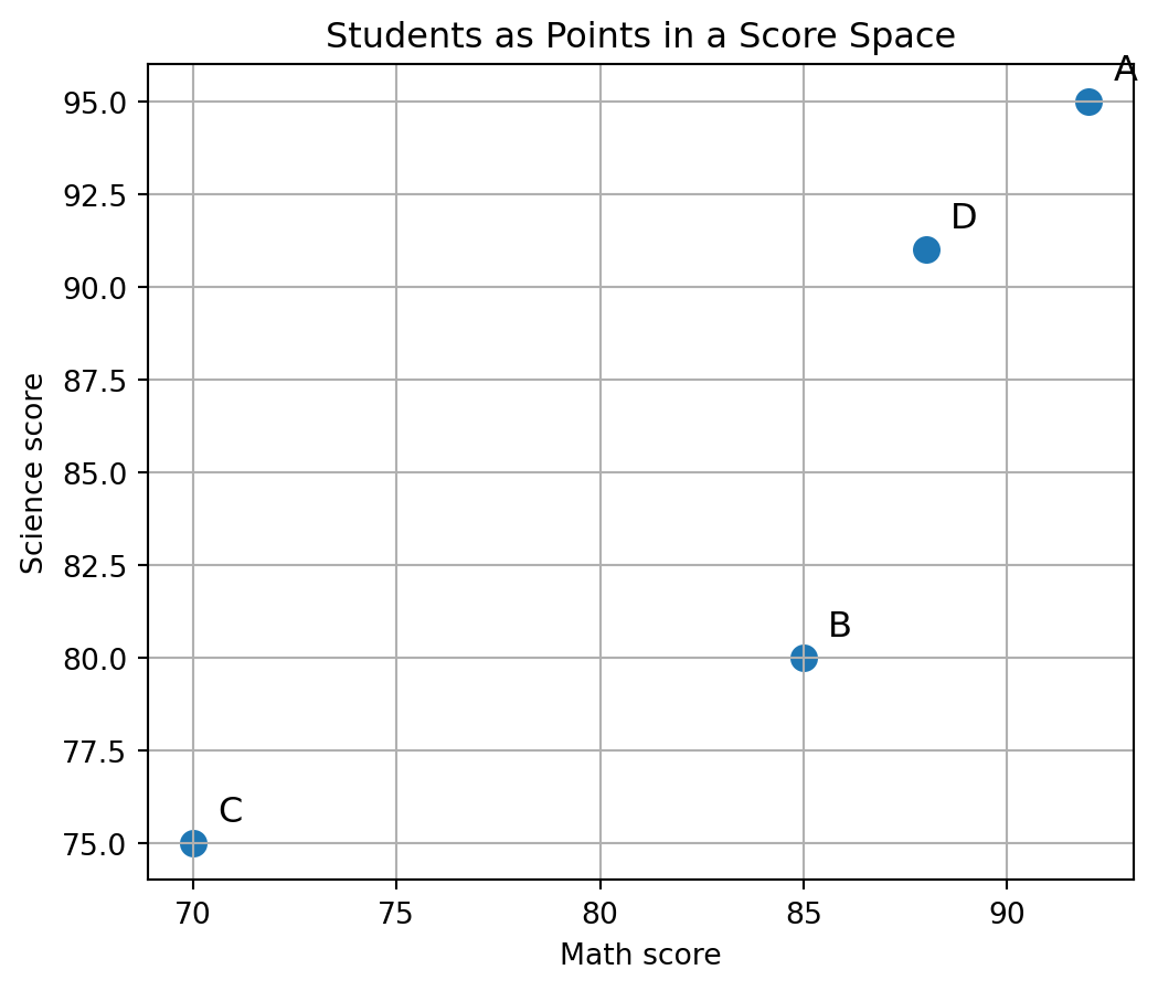
We can also visualize two features at a time:
```{python}
plt.figure(figsize=(6, 5))
plt.scatter(students["math"], students["science"], s=70)

for _, row in students.iterrows():
    plt.text(row["math"] + 0.6, row["science"] + 0.6, row["student"], fontsize=12)

plt.xlabel("Math score")
plt.ylabel("Science score")
plt.title("Students as Points in a Score Space")
plt.grid(True)
plt.show()
```
This simple example contains the basic pattern of many data projects:
1. choose features,
2. build vectors,
3. place the vectors in a data space,
4. compare or model the points.
## 1.15 A First Preview of the Book
This chapter is the first step in a longer story.
Once objects become vectors, we can ask deeper questions.
| Question | Linear Algebra Idea |
|---|---|
| How do we combine pieces of information? | vector addition and linear combinations |
| How do we transform data? | matrices as machines |
| How do we solve for unknowns? | linear systems |
| What happens when information is lost? | rank and null spaces |
| How do we measure similarity? | dot products and angles |
| How do we find the best approximation? | projections and least squares |
| What directions matter most? | eigenvectors and singular vectors |
| How do we compress images? | singular value decomposition |
| How do we represent text and AI models? | embeddings, matrices, and neural networks |
The whole book grows from the first translation:
$$
\text{object} \longrightarrow \text{vector}.
$$
## 1.16 Concept Summary
The central message of this chapter is:
> Linear algebra begins when we represent objects as vectors.
A vector is a list of coordinates. In applications, each coordinate has meaning. A data table is a collection of vectors. When objects become vectors, they become points in a feature space. Once objects are points, we can compare, visualize, transform, approximate, compress, and learn from them.
But representation is always a choice. It captures some information and ignores other information. Good linear algebra is not only about computation. It is also about understanding what the computation means.
## 1.17 Key Vocabulary
**Object**
Something we want to describe or study, such as a house, image, song, document, patient, student, or gene.
**Feature**
A measurable or encoded attribute of an object.
**Coordinate**
One entry of a vector.
**Vector**
An ordered list of numbers.
**Feature vector**
A vector whose coordinates represent features of an object.
**Feature map**
A rule or function that turns an object into a vector.
**Data point**
An object represented as a point in feature space.
**Feature space**
The coordinate space created by the chosen features.
**Data matrix**
A rectangular array whose rows often represent objects and whose columns represent features.
**High-dimensional data**
Data represented by vectors with many coordinates.
**Vectorization**
The process of turning an object into a vector.
**Scaling**
Changing feature values so that coordinates are measured on comparable numerical scales.
## 1.18 Practice Problems
### Problem 1: A Student as a Vector
Describe a student using a vector with four coordinates. State clearly what each coordinate means and what unit is used, if any.
<details>
<summary>Solution</summary>
One possible answer is
$$
x =
\begin{bmatrix}
90 \\
85 \\
12 \\
3
\end{bmatrix},
$$
where the coordinates mean
$$
\begin{bmatrix}
\text{math score} \\
\text{writing score} \\
\text{study hours per week} \\
\text{number of courses}
\end{bmatrix}.
$$
Many answers are possible. The important point is that each coordinate must have a clear interpretation.
</details>
### Problem 2: Interpret a Car Vector
A car is represented by
$$
x =
\begin{bmatrix}
30000 \\
35 \\
5 \\
2022
\end{bmatrix}.
$$
Give one possible meaning for each coordinate.
<details>
<summary>Solution</summary>
One possible interpretation is
$$
\begin{bmatrix}
\text{price in dollars} \\
\text{miles per gallon} \\
\text{number of seats} \\
\text{model year}
\end{bmatrix}
=
\begin{bmatrix}
30000 \\
35 \\
5 \\
2022
\end{bmatrix}.
$$
The same numerical vector could have other meanings if the coordinate dictionary changes.
</details>
### Problem 3: A Restaurant Vector
Suppose a restaurant is represented by
$$
\begin{bmatrix}
\text{price level} \\
\text{distance from campus} \\
\text{rating}
\end{bmatrix}.
$$
Write down a possible vector for a restaurant you know. Explain each coordinate.
<details>
<summary>Solution</summary>
A possible answer is
$$
\begin{bmatrix}
2 \\
0.8 \\
4.5
\end{bmatrix},
$$
where price level is on a scale from $1$ to $4$, distance is measured in miles, and rating is on a scale from $1$ to $5$.
</details>
### Problem 4: Text as a Vector
Use the vocabulary
$$
[\text{math}, \text{data}, \text{AI}, \text{model}].
$$
Write the word-count vector for the sentence:
> AI and data need a model.
Ignore words not in the vocabulary.
<details>
<summary>Solution</summary>
The sentence contains data once, AI once, and model once. It does not contain math. Therefore the vector is
$$
\begin{bmatrix}
0 \\
1 \\
1 \\
1
\end{bmatrix}.
$$
</details>
### Problem 5: Compare Movie Ratings
Suppose three users rate four movies:
$$
a =
\begin{bmatrix}
5 \\
4 \\
1 \\
1
\end{bmatrix},
\qquad
b =
\begin{bmatrix}
4 \\
5 \\
1 \\
2
\end{bmatrix},
\qquad
c =
\begin{bmatrix}
1 \\
1 \\
5 \\
5
\end{bmatrix}.
$$
Which user seems most similar to user $a$? Explain.
<details>
<summary>Solution</summary>
User $b$ seems most similar to user $a$. Their ratings are close in every coordinate. User $c$ has almost the opposite pattern: low ratings where $a$ has high ratings and high ratings where $a$ has low ratings.
Using distance:
$$
\|a-b\| = \sqrt{(5-4)^2+(4-5)^2+(1-1)^2+(1-2)^2}=\sqrt{3}.
$$
Also,
$$
\|a-c\| = \sqrt{(5-1)^2+(4-1)^2+(1-5)^2+(1-5)^2}=\sqrt{57}.
$$
Since $\sqrt{3}<\sqrt{57}$, $b$ is closer to $a$ than $c$ is.
</details>
### Problem 6: What Is Lost?
Choose one representation from this chapter: a house vector, image vector, text vector, or movie-rating vector. Write two things the representation captures and two things it loses.
<details>
<summary>Solution</summary>
For a house vector with size, bedrooms, distance, and price:
It captures size and price. It may also capture convenience through distance.
It loses information such as sunlight, noise, neighborhood feeling, layout, and emotional attachment.
</details>
## 1.19 Python Practice
### Exercise 1: Create a House Vector
Create a NumPy vector representing a house with features
$$
[\text{size}, \text{bedrooms}, \text{distance}, \text{price}].
$$
```{python}
house = np.array([1800, 3, 12, 550000])
house
```
### Exercise 2: Create Several Student Vectors
Create three student vectors using the features
$$
[\text{math score}, \text{writing score}, \text{science score}].
$$
Then compute the distance between two of them.
```{python}
student1 = np.array([90, 80, 85])
student2 = np.array([88, 82, 87])
student3 = np.array([60, 95, 70])

np.linalg.norm(student1 - student2), np.linalg.norm(student1 - student3)
```
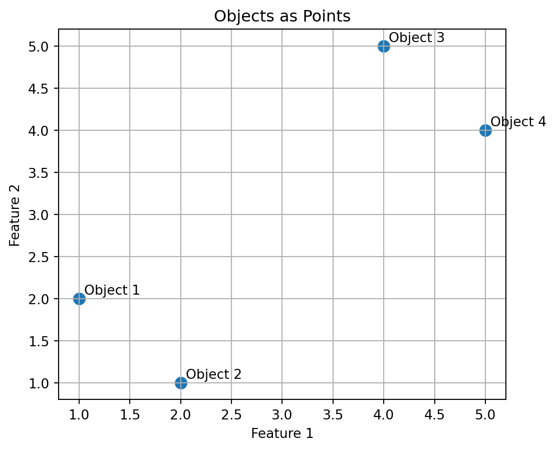
### Exercise 3: Plot Objects in Two-Dimensional Feature Space
```{python}
x_feature = np.array([1, 2, 4, 5])
y_feature = np.array([2, 1, 5, 4])
labels = ["Object 1", "Object 2", "Object 3", "Object 4"]

plt.figure(figsize=(6, 5))
plt.scatter(x_feature, y_feature, s=70)

for x, y, label in zip(x_feature, y_feature, labels):
    plt.text(x + 0.05, y + 0.05, label)

plt.xlabel("Feature 1")
plt.ylabel("Feature 2")
plt.title("Objects as Points")
plt.grid(True)
plt.show()
```
### Exercise 4: Compare Raw and Scaled Distances
```{python}
X = np.array([
    [1200, 400000],
    [1800, 550000],
    [2400, 610000],
    [1000, 420000]
])

raw_distance = np.linalg.norm(X[0] - X[1])

X_scaled = (X - X.mean(axis=0)) / X.std(axis=0)
scaled_distance = np.linalg.norm(X_scaled[0] - X_scaled[1])

raw_distance, scaled_distance
```
Think about why the two distances have different meanings.
### Exercise 5: One-Hot Encoding
Represent the heating types gas, electric, and oil using one-hot vectors.
```{python}
heating_to_vector = {
    "gas": np.array([1, 0, 0]),
    "electric": np.array([0, 1, 0]),
    "oil": np.array([0, 0, 1])
}

heating_to_vector["gas"]
```
## 1.20 Challenge Questions
### Challenge 1: Is Bigger Always Better?
Suppose two features are income and age. Income may be measured in dollars, while age is measured in years. Explain why direct distance between vectors may be misleading.
<details>
<summary>Solution</summary>
Income values may be in the tens of thousands or hundreds of thousands, while age values may be between about $0$ and $100$. A direct distance calculation may be dominated by income because its numerical scale is much larger. This does not automatically mean income is more important. It may only mean income is measured in larger units.
</details>
### Challenge 2: Two Different Feature Maps
Give two different feature maps for the same object: a song. Explain what each feature map is useful for.
<details>
<summary>Solution</summary>
One feature map could describe a song by audio properties:
$$
\begin{bmatrix}
\text{tempo} \\
\text{loudness} \\
\text{duration} \\
\text{average pitch}
\end{bmatrix}.
$$
This may be useful for audio analysis.
Another feature map could describe listener behavior:
$$
\begin{bmatrix}
\text{number of plays} \\
\text{number of skips} \\
\text{number of likes} \\
\text{playlist appearances}
\end{bmatrix}.
$$
This may be useful for recommendation systems.
</details>
### Challenge 3: Can a Bad Representation Give a Bad Answer?
Explain why a machine learning model can fail if the vector representation ignores important information.
<details>
<summary>Solution</summary>
A model can only use the information present in the vectors. If the representation omits important features, the model may make predictions from incomplete or misleading information. For example, a house-price model that ignores location may perform poorly because location strongly affects price.
</details>
## 1.21 AI Companion Activities
Use an AI tool as a learning companion. Do not only copy its answer. Question it, improve it, and connect it to the ideas in this chapter.
### Activity 1: Real-World Vectors
Ask:
> Give me ten examples of real-world objects that can be represented as vectors. For each example, list possible coordinates and units.
Choose three examples and improve the coordinate choices.
### Activity 2: What Is Lost?
Ask:
> If a person is represented by height, weight, age, and income, what information is captured and what information is lost?
Then write your own response. Be specific about what the vector can and cannot say.
### Activity 3: Better Feature Maps
Ask:
> Give two different feature maps for the same object, such as a song, a house, or a medical patient. Explain how the purpose changes the feature map.
Compare the AI's answer with the feature-map idea in Section 1.4.
### Activity 4: Scaling and Units
Ask:
> Explain why feature scaling matters when comparing vectors by distance. Give a simple numerical example.
Then create your own example with two features measured in very different units.
## 1.22 Reflection Questions
1. Why is a vector more than just a list of numbers?
2. Why does every coordinate need interpretation?
3. What is a feature map?
4. How is a data table related to a collection of vectors?
5. Why is high-dimensional data natural in modern applications?
6. What is one advantage of representing objects as vectors?
7. What is one danger of representing objects as vectors?
8. Why can units change geometric comparisons?
9. Give an example where a vector captures useful information but loses something important.
10. How does the idea "objects become vectors" prepare us for the rest of linear algebra?
## 1.23 Chapter Closing: The First Translation
Linear algebra begins with a translation.
The world gives us houses, images, songs, documents, students, patients, markets, genes, and conversations.
Mathematics asks us to choose features.
Computation asks us to store those features as numbers.
Geometry asks us to see the resulting vectors as points in a space.
This first translation is simple, but it changes everything:
$$
\text{world} \longrightarrow \text{features} \longrightarrow \text{vectors} \longrightarrow \text{geometry}.
$$
A vector is not the whole object. It is a carefully chosen numerical shadow. Once we have that shadow, linear algebra gives us a way to compare, combine, transform, compress, approximate, and learn.
In the next chapter, we study vectors themselves more deeply. We will see that a vector can be a point, an arrow, a movement, a feature list, or a package of information.
The story of linear algebra has begun.