---
title: "Chapter 7: Solving Backwards"
subtitle: "Linear systems as reverse engineering"
format:
html:
toc: true
toc-depth: 3
number-sections: true
code-fold: true
code-tools: true
jupyter: python3
---
## Opening Story: The Recipe Hidden Inside the Result
A matrix can be a machine.
In the previous chapters, we learned how a matrix takes an input vector and produces an output vector. We watched grids stretch, rotate, shear, reflect, and sometimes collapse. That was the **forward problem**:
$$
\text{input} \longrightarrow \text{matrix machine} \longrightarrow \text{output}.
$$
But much of science, data analysis, engineering, economics, and artificial intelligence begins with the opposite question.
We see the output.
We know something about the machine.
We want to recover the input.
That is the **backward problem**.
Imagine a smoothie bar. The machine mixes two ingredients: banana and strawberry. The output has two measured properties: sweetness and thickness. Suppose the machine follows the rule
$$
\begin{bmatrix}
\text{sweetness} \\
\text{thickness}
\end{bmatrix}
=
\begin{bmatrix}
2 & 1 \\
1 & 3
\end{bmatrix}
\begin{bmatrix}
\text{banana} \\
\text{strawberry}
\end{bmatrix}.
$$
If we put in $2$ units of banana and $3$ units of strawberry, the output is
$$
\begin{bmatrix}
2 & 1 \\
1 & 3
\end{bmatrix}
\begin{bmatrix}
2 \\
3
\end{bmatrix}
=
\begin{bmatrix}
7 \\
11
\end{bmatrix}.
$$
Now reverse the question:
> If we want sweetness $7$ and thickness $11$, what ingredients should we put in?
In symbols, we want to solve
$$
\begin{bmatrix}
2 & 1 \\
1 & 3
\end{bmatrix}
\begin{bmatrix}
x_1 \\
x_2
\end{bmatrix}
=
\begin{bmatrix}
7 \\
11
\end{bmatrix}.
$$
This is a **linear system**. It asks us to run a matrix machine backwards.
::: {.callout-important}
## Main Message
A linear system
$$
Ax=b
$$
asks:
> Which input vector $x$ does the matrix machine $A$ send to the target output vector $b$?
Solving a system is reverse engineering.
:::
## Learning Goals
By the end of this chapter, you should be able to:
1. Translate a system of equations into matrix form $Ax=b$.
2. Interpret solving as running a matrix machine backwards.
3. Explain the equation picture, line picture, row picture, and column picture of a system.
4. Use elimination and row operations to solve small systems.
5. Distinguish between one solution, no solution, and infinitely many solutions.
6. Explain consistency, reachability, and information loss.
7. Use Python to solve and diagnose linear systems.
8. Understand why numerical linear algebra is more than pressing `solve`.
## 7.1 The Forward Problem and the Backward Problem
Let
$$
A=
\begin{bmatrix}
2 & 1 \\
1 & 3
\end{bmatrix},
\qquad
x=
\begin{bmatrix}
2 \\
3
\end{bmatrix}.
$$
The forward problem is easy:
$$
b=Ax
=
\begin{bmatrix}
2 & 1 \\
1 & 3
\end{bmatrix}
\begin{bmatrix}
2 \\
3
\end{bmatrix}
=
\begin{bmatrix}
7 \\
11
\end{bmatrix}.
$$
The backward problem begins with $A$ and $b$ and asks for $x$:
$$
Ax=b.
$$
For this example,
$$
\begin{bmatrix}
2 & 1 \\
1 & 3
\end{bmatrix}
\begin{bmatrix}
x_1 \\
x_2
\end{bmatrix}
=
\begin{bmatrix}
7 \\
11
\end{bmatrix}.
$$
Multiplying out gives
$$
2x_1+x_2=7,
$$
$$
x_1+3x_2=11.
$$
So a matrix equation is a compact way to write a system of equations.
::: {.callout-note}
## Four Ways to See $Ax=b$
The same system has several meanings:
| View | Interpretation |
|---|---|
| Machine view | Find the input that produces the output. |
| Equation view | Find numbers satisfying all equations at once. |
| Geometry view | Find intersections of lines, planes, or higher-dimensional flats. |
| Column view | Build $b$ as a linear combination of the columns of $A$. |
:::
## 7.2 Systems as Intersections
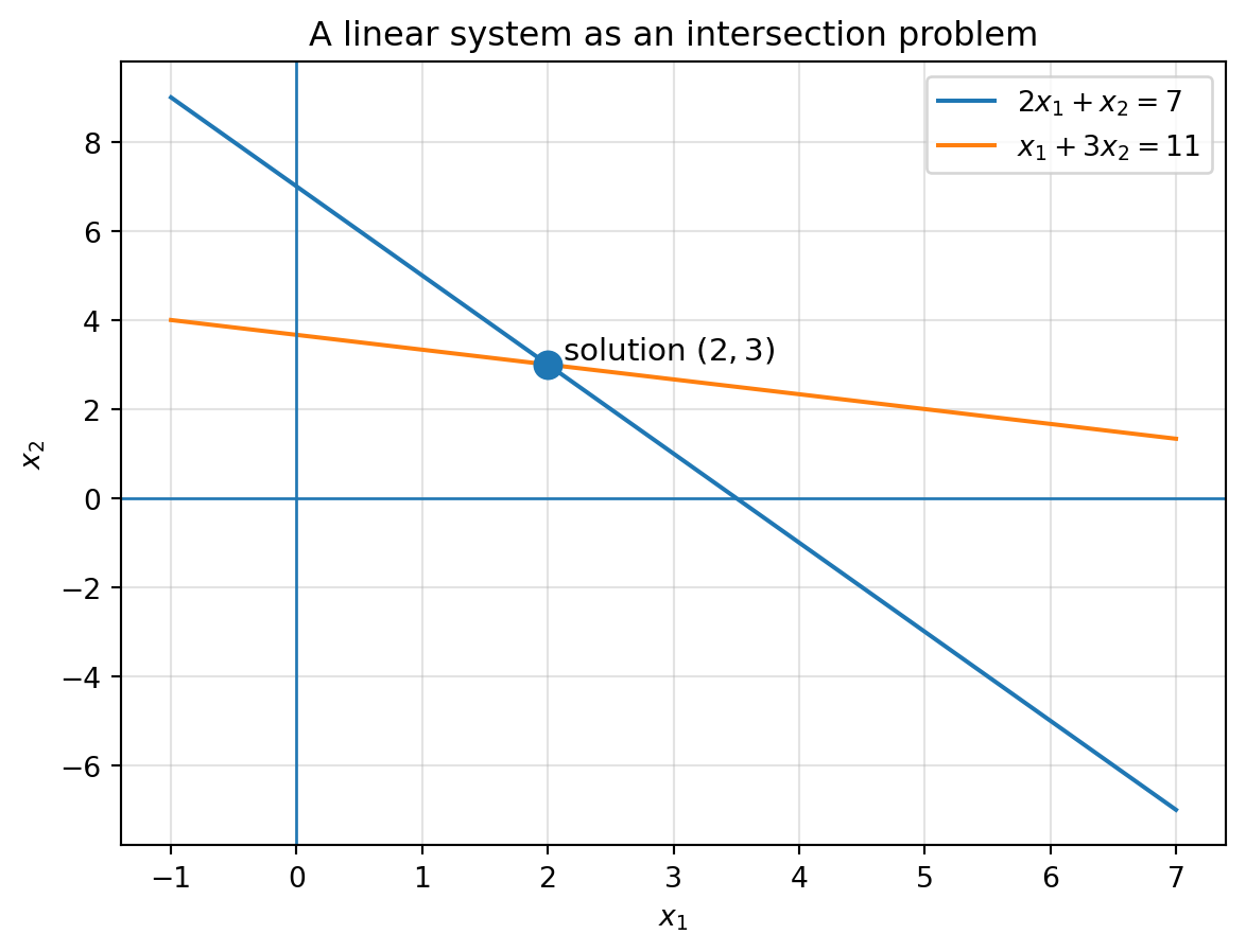
The equations
$$
2x_1+x_2=7,
\qquad
x_1+3x_2=11
$$
describe two lines in the plane. The solution is the point where the two lines meet.
```{python}
import numpy as np
import matplotlib.pyplot as plt

x = np.linspace(-1, 7, 400)
y1 = 7 - 2*x
y2 = (11 - x)/3

plt.figure(figsize=(7, 5))
plt.plot(x, y1, label="$2x_1+x_2=7$")
plt.plot(x, y2, label="$x_1+3x_2=11$")
plt.scatter([2], [3], s=90, zorder=5)
plt.text(2.12, 3.12, "solution $(2,3)$", fontsize=11)
plt.axhline(0, linewidth=1)
plt.axvline(0, linewidth=1)
plt.xlabel("$x_1$")
plt.ylabel("$x_2$")
plt.title("A linear system as an intersection problem")
plt.grid(True, alpha=0.35)
plt.legend()
plt.show()
```
The intersection is $(2,3)$, so
$$
x=
\begin{bmatrix}
2 \\
3
\end{bmatrix}.
$$
This picture is helpful, but it is also limited. In three unknowns, equations become planes. In one hundred unknowns, we cannot draw the picture. The ideas still work, but we need algebra and computation.
## 7.3 Substitution: Solving by Rewriting
For small systems, substitution is natural.
Start with
$$
2x_1+x_2=7,
\qquad
x_1+3x_2=11.
$$
From the first equation,
$$
x_2=7-2x_1.
$$
Substitute into the second equation:
$$
x_1+3(7-2x_1)=11.
$$
Then
$$
x_1+21-6x_1=11,
$$
so
$$
-5x_1=-10,
\qquad
x_1=2.
$$
Then
$$
x_2=7-2(2)=3.
$$
Substitution is useful for understanding, but it does not scale well. For larger systems, we need a method that is organized enough for machines.
## 7.4 Elimination: Removing One Unknown at a Time
Elimination solves a system by combining equations to remove variables.
Start again:
$$
2x_1+x_2=7,
$$
$$
x_1+3x_2=11.
$$
Multiply the second equation by $2$:
$$
2x_1+6x_2=22.
$$
Subtract the first equation:
$$
(2x_1+6x_2)-(2x_1+x_2)=22-7.
$$
Thus
$$
5x_2=15,
\qquad
x_2=3.
$$
Then
$$
2x_1+3=7,
\qquad
x_1=2.
$$
Elimination is the beginning of **Gaussian elimination**, one of the central algorithms of linear algebra.
## 7.5 The Augmented Matrix
To eliminate efficiently, we stop rewriting the variable names and keep only the coefficients.
The system
$$
2x_1+x_2=7,
\qquad
x_1+3x_2=11
$$
becomes the augmented matrix
$$
\left[
\begin{array}{cc|c}
2 & 1 & 7 \\
1 & 3 & 11
\end{array}
\right].
$$
The left block is $A$. The right column is $b$. The vertical bar is a visual separator.
::: {.callout-tip}
## Reading an Augmented Matrix
$$
\left[\begin{array}{ccc|c}
a_{11} & a_{12} & a_{13} & b_1 \\
a_{21} & a_{22} & a_{23} & b_2
\end{array}\right]
$$
means
$$
a_{11}x_1+a_{12}x_2+a_{13}x_3=b_1,
$$
$$
a_{21}x_1+a_{22}x_2+a_{23}x_3=b_2.
$$
:::
## 7.6 Row Operations Preserve the Solution Set
Elimination uses three legal row operations:
1. Swap two rows.
2. Multiply a row by a nonzero scalar.
3. Add a multiple of one row to another row.
These operations change the appearance of the equations, but not the set of solutions.
Why?
Because each operation replaces the system by an equivalent description of the same restrictions.
::: {.callout-important}
## Row Operations Preserve Solutions
Legal row operations preserve the solution set. They do not change which vectors $x$ satisfy the system.
They only change the system into an easier form.
:::
## 7.7 Row Reduction Example
Start with
$$
\left[
\begin{array}{cc|c}
2 & 1 & 7 \\
1 & 3 & 11
\end{array}
\right].
$$
Swap rows:
$$
\left[
\begin{array}{cc|c}
1 & 3 & 11 \\
2 & 1 & 7
\end{array}
\right].
$$
Replace Row 2 by Row 2 minus $2$ times Row 1:
$$
\left[
\begin{array}{cc|c}
1 & 3 & 11 \\
0 & -5 & -15
\end{array}
\right].
$$
Divide Row 2 by $-5$:
$$
\left[
\begin{array}{cc|c}
1 & 3 & 11 \\
0 & 1 & 3
\end{array}
\right].
$$
Replace Row 1 by Row 1 minus $3$ times Row 2:
$$
\left[
\begin{array}{cc|c}
1 & 0 & 2 \\
0 & 1 & 3
\end{array}
\right].
$$
Now the solution is visible:
$$
x_1=2,
\qquad
x_2=3.
$$
## 7.8 Pivots: The Places Where Solving Gets Control
During elimination, a **pivot** is the leading nonzero entry used to eliminate entries below or above it.
Pivots are the places where the system gives independent information.
For the matrix
$$
\begin{bmatrix}
2 & 1 \\
1 & 3
\end{bmatrix},
$$
there are two pivots. That means the two variables are controlled uniquely.
For
$$
\begin{bmatrix}
1 & 1 \\
2 & 2
\end{bmatrix},
$$
there is only one pivot. The second equation repeats the first. One variable remains free.
This pivot language will become essential when we study rank, null space, column space, and invertibility.
## 7.9 Three Possible Outcomes
A linear system may have:
1. exactly one solution,
2. no solution,
3. infinitely many solutions.
For two equations in two unknowns, the geometry is easy to draw.
| Geometry | Algebraic meaning | Number of solutions |
|---|---|---|
| Lines intersect once | Two independent equations | One solution |
| Lines are parallel and distinct | Contradictory equations | No solution |
| Lines are the same | One equation repeats the other | Infinitely many solutions |
But the same logic continues in higher dimensions.
## 7.10 One Solution
The system
$$
2x_1+x_2=7,
\qquad
x_1+3x_2=11
$$
has one solution because the two equations give two independent restrictions. Geometrically, the lines meet once. Algebraically, both variables are controlled.
For a square system, one solution is connected to an invertible matrix.
## 7.11 No Solution
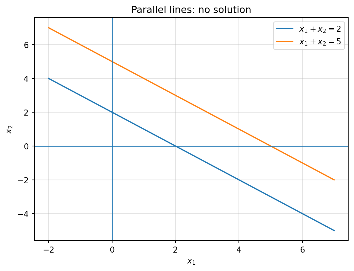
Consider
$$
x_1+x_2=2,
$$
$$
x_1+x_2=5.
$$
The same left side cannot equal both $2$ and $5$. The equations contradict each other.
```{python}
x = np.linspace(-2, 7, 400)
y1 = 2 - x
y2 = 5 - x

plt.figure(figsize=(7, 5))
plt.plot(x, y1, label="$x_1+x_2=2$")
plt.plot(x, y2, label="$x_1+x_2=5$")
plt.axhline(0, linewidth=1)
plt.axvline(0, linewidth=1)
plt.xlabel("$x_1$")
plt.ylabel("$x_2$")
plt.title("Parallel lines: no solution")
plt.grid(True, alpha=0.35)
plt.legend()
plt.show()
```
The system is **inconsistent**.
::: {.callout-warning}
## No Solution Means Unreachable
In the equation $Ax=b$, no solution means that the target vector $b$ is not reachable from the columns of $A$.
:::
## 7.12 Infinitely Many Solutions
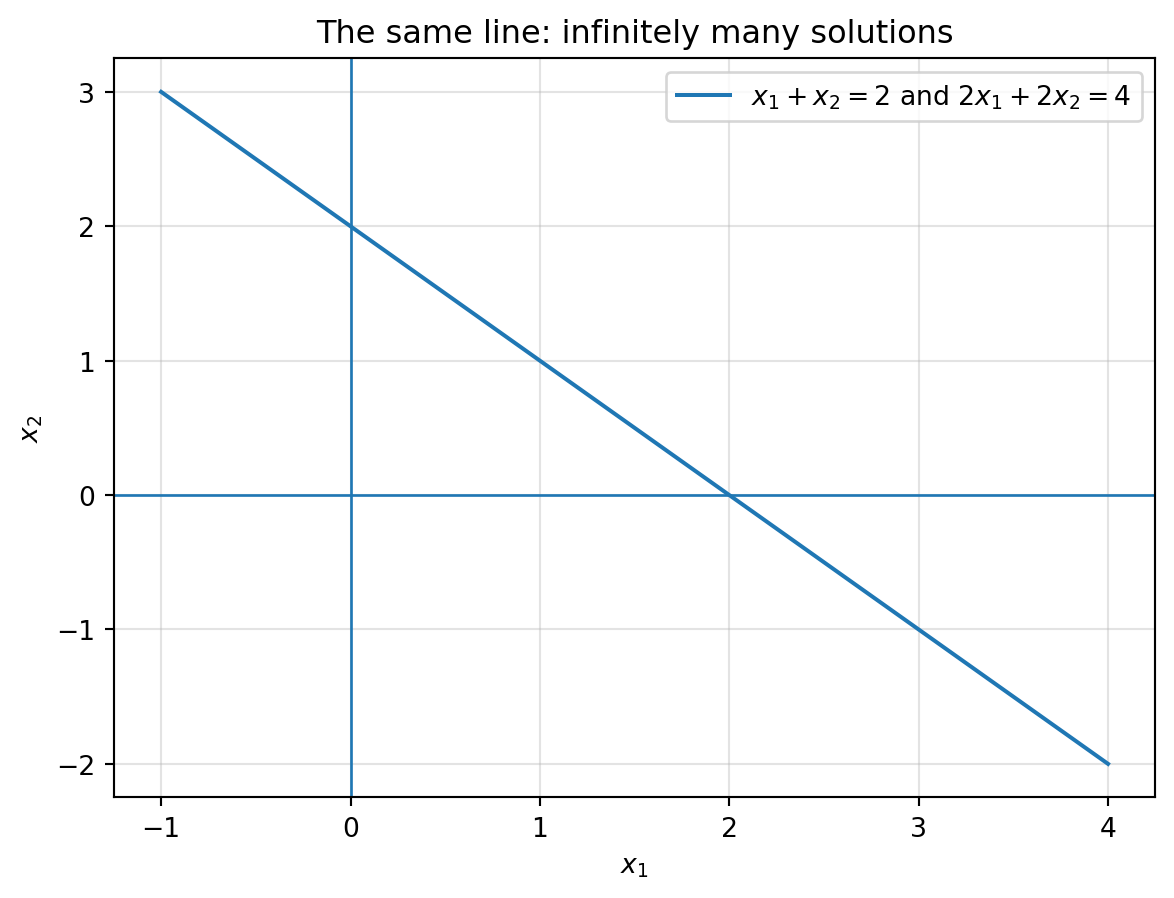
Consider
$$
x_1+x_2=2,
$$
$$
2x_1+2x_2=4.
$$
The second equation is just twice the first. Both equations describe the same line.
```{python}
x = np.linspace(-1, 4, 400)
y = 2 - x

plt.figure(figsize=(7, 5))
plt.plot(x, y, label="$x_1+x_2=2$ and $2x_1+2x_2=4$")
plt.axhline(0, linewidth=1)
plt.axvline(0, linewidth=1)
plt.xlabel("$x_1$")
plt.ylabel("$x_2$")
plt.title("The same line: infinitely many solutions")
plt.grid(True, alpha=0.35)
plt.legend()
plt.show()
```
Every point on the line $x_1+x_2=2$ is a solution:
$$
\begin{bmatrix}
2 \\
0
\end{bmatrix},
\quad
\begin{bmatrix}
1 \\
1
\end{bmatrix},
\quad
\begin{bmatrix}
0 \\
2
\end{bmatrix},
\quad
\begin{bmatrix}
t \\
2-t
\end{bmatrix}.
$$
Infinitely many solutions mean that the matrix machine loses information: different inputs produce the same output.
## 7.13 Consistency and Reachability
A system $Ax=b$ is **consistent** if it has at least one solution.
It is **inconsistent** if it has no solution.
The column picture gives the most important interpretation:
$$
Ax=b
$$
means
$$
x_1a_1+x_2a_2+\cdots+x_na_n=b,
$$
where $a_1,a_2,\ldots,a_n$ are the columns of $A$.
So solving $Ax=b$ asks:
> Can we build $b$ from the columns of $A$?
If yes, the system is consistent. If no, it is inconsistent.
::: {.callout-important}
## Column Picture of Solving
Solving $Ax=b$ means asking whether $b$ lies in the span of the columns of $A$.
If $b$ is in the span, a solution vector $x$ gives the recipe for building $b$ from the columns.
:::
## 7.14 Column Picture Example
Let
$$
A=
\begin{bmatrix}
2 & 1 \\
1 & 3
\end{bmatrix},
\qquad
b=
\begin{bmatrix}
7 \\
11
\end{bmatrix}.
$$
The columns of $A$ are
$$
a_1=
\begin{bmatrix}
2 \\
1
\end{bmatrix},
\qquad
a_2=
\begin{bmatrix}
1 \\
3
\end{bmatrix}.
$$
Solving $Ax=b$ means finding coefficients $x_1$ and $x_2$ such that
$$
x_1a_1+x_2a_2=b.
$$
The solution is
$$
x_1=2,
\qquad
x_2=3,
$$
because
$$
2\begin{bmatrix}
2 \\
1
\end{bmatrix}
+
3\begin{bmatrix}
1 \\
3
\end{bmatrix}
=
\begin{bmatrix}
7 \\
11
\end{bmatrix}.
$$
The solution vector is not just two numbers. It is a recipe.
## 7.15 A Machine That Loses Information
Consider
$$
A=
\begin{bmatrix}
1 & 1 \\
2 & 2
\end{bmatrix}.
$$
The columns are identical:
$$
a_1=a_2=
\begin{bmatrix}
1 \\
2
\end{bmatrix}.
$$
Then
$$
Ax=x_1a_1+x_2a_2=(x_1+x_2)a_1.
$$
Only the sum $x_1+x_2$ matters. The individual values are not remembered.
For example,
$$
\begin{bmatrix}
2 \\
0
\end{bmatrix},
\quad
\begin{bmatrix}
1 \\
1
\end{bmatrix},
\quad
\begin{bmatrix}
0 \\
2
\end{bmatrix}
$$
all produce
$$
\begin{bmatrix}
2 \\
4
\end{bmatrix}.
$$
This is the beginning of null-space thinking: some directions in input space become invisible in output space.
## 7.16 Invertible Machines
A square matrix is **invertible** when its machine can be reversed perfectly.
For a square matrix $A$, invertibility means:
1. Every output vector $b$ is reachable.
2. Every output vector $b$ has exactly one input $x$.
3. The equation $Ax=b$ has a unique solution for every $b$.
4. The matrix does not collapse information.
::: {.callout-note}
## Invertible Matrix
A square matrix $A$ is invertible if, for every output vector $b$, there is exactly one input vector $x$ such that $Ax=b$.
:::
We will study invertibility more deeply later. For now, remember the story:
> Invertible means the machine can be run backwards without ambiguity.
## 7.17 Python: Solving a Linear System
Use `np.linalg.solve(A, b)` when $A$ is square and invertible.
```{python}
import numpy as np

A = np.array([
    [2, 1],
    [1, 3]
], dtype=float)

b = np.array([7, 11], dtype=float)

x = np.linalg.solve(A, b)
x
```
Check the result:
```{python}
A @ x
```
Check the residual:
```{python}
r = b - A @ x
np.linalg.norm(r)
```
The **residual** $r=b-Ax$ measures what is left unexplained. For an exact solution, the residual is zero, up to small numerical roundoff.
## 7.18 Python: Diagnosing Singular Systems
A singular matrix cannot be inverted. This does not automatically mean the system has no solution. It means the backward problem is not uniquely solvable.
Consider
$$
A=
\begin{bmatrix}
1 & 1 \\
2 & 2
\end{bmatrix}.
$$
```{python}
A = np.array([
    [1, 1],
    [2, 2]
], dtype=float)

np.linalg.det(A)
```
The determinant is zero, so the matrix collapses area and loses information.
If
$$
b=\begin{bmatrix}2 \\ 4\end{bmatrix},
$$
the system has infinitely many solutions.
If
$$
b=\begin{bmatrix}2 \\ 5\end{bmatrix},
$$
the system has no solution.
```{python}
for b in [np.array([2, 4], dtype=float), np.array([2, 5], dtype=float)]:
    x_lstsq, residuals, rank, s = np.linalg.lstsq(A, b, rcond=None)
    print("b =", b)
    print("least-squares x =", x_lstsq)
    print("A @ x =", A @ x_lstsq)
    print("residual norm =", np.linalg.norm(b - A @ x_lstsq))
    print("rank =", rank)
    print()
```
The same singular matrix can produce different stories depending on $b$.
## 7.19 Why `solve` Is Not the Same as Understanding
Python can compute quickly, but we must still ask mathematical questions:
- Is $A$ square?
- Is $A$ invertible?
- Is the system consistent?
- Is the solution unique?
- Is the answer numerically stable?
- Does the solution make sense in the original problem?
A computer can give numbers. Linear algebra tells us what the numbers mean.
## 7.20 Application: Prices from Purchases
A store sells apples and bananas.
One customer buys $2$ apples and $1$ banana for $5.00$.
Another customer buys $1$ apple and $3$ bananas for $8.00$.
Let
$$
a=\text{price of one apple},
\qquad
b=\text{price of one banana}.
$$
Then
$$
2a+b=5,
\qquad
a+3b=8.
$$
In matrix form,
$$
\begin{bmatrix}
2 & 1 \\
1 & 3
\end{bmatrix}
\begin{bmatrix}
a \\
b
\end{bmatrix}
=
\begin{bmatrix}
5 \\
8
\end{bmatrix}.
$$
```{python}
A = np.array([
    [2, 1],
    [1, 3]
], dtype=float)

b = np.array([5, 8], dtype=float)

prices = np.linalg.solve(A, b)
prices
```
The solution gives the hidden unit prices.
This is the central pattern of solving backwards:
> Totals are visible. Components are hidden. Linear algebra recovers the components.
## 7.21 Application: Mixtures and Sensors
Suppose two sensors measure two hidden signals. The measurements are mixtures:
$$
y_1=0.8s_1+0.3s_2,
$$
$$
y_2=0.2s_1+0.9s_2.
$$
In matrix form,
$$
y=As,
\qquad
A=
\begin{bmatrix}
0.8 & 0.3 \\
0.2 & 0.9
\end{bmatrix}.
$$
If we observe $y$, can we recover $s$?
```{python}
A = np.array([
    [0.8, 0.3],
    [0.2, 0.9]
])

s_true = np.array([3.0, 5.0])
y = A @ s_true
s_recovered = np.linalg.solve(A, y)

y, s_recovered
```
This tiny example is a toy version of signal separation, imaging, and inverse problems.
## 7.22 High-Dimensional Systems
In real applications, systems may have thousands or millions of variables.
A recommendation system may solve for hidden user preferences.
A CT scanner may solve for internal densities of the body.
A machine learning model may solve for weights that match data.
A network problem may solve for flows through many edges.
The equation still has the same shape:
$$
Ax=b.
$$
The story does not change. Only the size changes.
```{python}
np.random.seed(7)

n = 80
A = np.random.randn(n, n)
x_true = np.random.randn(n)
b = A @ x_true

x_recovered = np.linalg.solve(A, b)
error = np.linalg.norm(x_recovered - x_true)
residual = np.linalg.norm(A @ x_recovered - b)

error, residual
```
In exact mathematics, the recovered solution equals the true solution. In floating-point computation, we expect tiny errors due to numerical roundoff.
## 7.23 Concept Summary
A linear system
$$
Ax=b
$$
means:
> Find the input vector $x$ that the matrix $A$ sends to the output vector $b$.
The most important interpretations are:
| View | Meaning |
|---|---|
| Machine view | Run the matrix machine backwards. |
| Equation view | Satisfy several equations at once. |
| Geometry view | Find an intersection. |
| Row view | Simplify equations without changing solutions. |
| Column view | Build $b$ from the columns of $A$. |
| Data view | Recover hidden quantities from observed totals. |
The solution set can have one solution, no solution, or infinitely many solutions.
## 7.24 Key Vocabulary
**Linear system**
A collection of linear equations.
**Matrix equation**
An equation of the form $Ax=b$.
**Coefficient matrix**
The matrix $A$ containing the coefficients of the system.
**Unknown vector**
The vector $x$ we want to find.
**Target vector**
The vector $b$ we want to produce.
**Augmented matrix**
A matrix that stores $A$ and $b$ together.
**Row operation**
A legal operation that preserves the solution set.
**Elimination**
A systematic method for simplifying a system.
**Pivot**
A leading nonzero entry used to control a variable during elimination.
**Consistent system**
A system with at least one solution.
**Inconsistent system**
A system with no solution.
**Singular matrix**
A square matrix that is not invertible.
**Invertible matrix**
A square matrix whose machine can be reversed uniquely.
**Residual**
The vector $b-Ax$, measuring how far $x$ is from solving the system exactly.
## 7.25 Worked Examples
### Example 1: Solve a System
Solve
$$
3x_1+2x_2=12,
$$
$$
x_1-x_2=1.
$$
::: {.callout-caution collapse="true"}
## Solution
From the second equation, $x_1=1+x_2$. Substitute into the first:
$$
3(1+x_2)+2x_2=12.
$$
So
$$
3+5x_2=12,
\qquad
x_2=\frac{9}{5}.
$$
Then
$$
x_1=1+\frac{9}{5}=\frac{14}{5}.
$$
Thus
$$
x=\begin{bmatrix}14/5 \\ 9/5\end{bmatrix}.
$$
:::
### Example 2: Diagnose the System
Consider
$$
x_1+2x_2=4,
$$
$$
2x_1+4x_2=9.
$$
::: {.callout-caution collapse="true"}
## Solution
The left side of the second equation is twice the left side of the first, but the right side is not twice $4$.
If the first equation is true, then
$$
2x_1+4x_2=8.
$$
But the second equation demands
$$
2x_1+4x_2=9.
$$
This is impossible. The system has no solution.
:::
### Example 3: Column Recipe
Let
$$
A=\begin{bmatrix}1 & 2 \\ 3 & 1\end{bmatrix},
\qquad
b=\begin{bmatrix}8 \\ 13\end{bmatrix}.
$$
Solve $Ax=b$ and interpret the answer as a column recipe.
::: {.callout-caution collapse="true"}
## Solution
We solve
$$
x_1\begin{bmatrix}1 \\ 3\end{bmatrix}
+x_2\begin{bmatrix}2 \\ 1\end{bmatrix}
=
\begin{bmatrix}8 \\ 13\end{bmatrix}.
$$
The equations are
$$
x_1+2x_2=8,
$$
$$
3x_1+x_2=13.
$$
From the first equation, $x_1=8-2x_2$. Substitute:
$$
3(8-2x_2)+x_2=13,
$$
so
$$
24-5x_2=13,
\qquad
x_2=\frac{11}{5}.
$$
Then
$$
x_1=8-2\cdot \frac{11}{5}=\frac{18}{5}.
$$
Thus
$$
\frac{18}{5}\begin{bmatrix}1 \\ 3\end{bmatrix}
+
\frac{11}{5}\begin{bmatrix}2 \\ 1\end{bmatrix}
=
\begin{bmatrix}8 \\ 13\end{bmatrix}.
$$
:::
## 7.26 Practice Problems
### Problem 1
Write the system
$$
4x_1-x_2=6,
$$
$$
2x_1+3x_2=13
$$
in matrix form $Ax=b$.
::: {.callout-caution collapse="true"}
## Solution
$$
\begin{bmatrix}
4 & -1 \\
2 & 3
\end{bmatrix}
\begin{bmatrix}
x_1 \\
x_2
\end{bmatrix}
=
\begin{bmatrix}
6 \\
13
\end{bmatrix}.
$$
:::
### Problem 2
Solve
$$
2x_1+x_2=9,
$$
$$
x_1+x_2=5.
$$
::: {.callout-caution collapse="true"}
## Solution
Subtract the second equation from the first:
$$
x_1=4.
$$
Then
$$
4+x_2=5,
$$
so $x_2=1$. Thus
$$
x=\begin{bmatrix}4 \\ 1\end{bmatrix}.
$$
:::
### Problem 3
For the system
$$
x_1+x_2=3,
$$
$$
2x_1+2x_2=6,
$$
explain why there are infinitely many solutions. Give three solutions.
::: {.callout-caution collapse="true"}
## Solution
The second equation is twice the first, so it gives no new restriction. The solutions are all points satisfying $x_1+x_2=3$.
Three examples are
$$
\begin{bmatrix}3 \\ 0\end{bmatrix},
\quad
\begin{bmatrix}2 \\ 1\end{bmatrix},
\quad
\begin{bmatrix}0 \\ 3\end{bmatrix}.
$$
:::
### Problem 4
For the system
$$
x_1+x_2=3,
$$
$$
x_1+x_2=7,
$$
explain why there is no solution.
::: {.callout-caution collapse="true"}
## Solution
The same quantity $x_1+x_2$ cannot equal both $3$ and $7$. The system is inconsistent.
:::
### Problem 5
Let
$$
A=\begin{bmatrix}1 & 2 \\ 3 & 4\end{bmatrix},
\qquad
b=\begin{bmatrix}5 \\ 11\end{bmatrix}.
$$
Solve $Ax=b$.
::: {.callout-caution collapse="true"}
## Solution
The equations are
$$
x_1+2x_2=5,
$$
$$
3x_1+4x_2=11.
$$
From the first equation, $x_1=5-2x_2$. Substitute:
$$
3(5-2x_2)+4x_2=11.
$$
So
$$
15-2x_2=11,
\qquad
x_2=2.
$$
Then $x_1=1$. Thus
$$
x=\begin{bmatrix}1 \\ 2\end{bmatrix}.
$$
:::
### Problem 6
Explain the column picture of solving $Ax=b$ in your own words.
::: {.callout-caution collapse="true"}
## Sample Answer
The columns of $A$ are building blocks. Solving $Ax=b$ asks whether the target vector $b$ can be built as a linear combination of those columns. The entries of $x$ are the coefficients in the recipe.
:::
### Problem 7
Create your own real-world reverse problem that leads to a $2\times 2$ linear system. Write the system and interpret the unknowns.
::: {.callout-caution collapse="true"}
## Sample Answer
Suppose one bundle has $3$ notebooks and $2$ pens and costs $11$, while another bundle has $1$ notebook and $4$ pens and costs $9$. If $n$ is notebook price and $p$ is pen price, then
$$
3n+2p=11,
\qquad
n+4p=9.
$$
The unknowns are unit prices.
:::
## 7.27 Python Practice
### Exercise 1: Solve and Check
```{python}
A = np.array([
    [2, 1],
    [1, 1]
], dtype=float)

b = np.array([9, 5], dtype=float)

x = np.linalg.solve(A, b)
print(x)
print(A @ x)
print("residual norm:", np.linalg.norm(b - A @ x))
```
### Exercise 2: Create a System from a Known Solution
```{python}
A = np.array([
    [3, 1],
    [2, 4]
], dtype=float)

x_true = np.array([2, 5], dtype=float)
b = A @ x_true

x_recovered = np.linalg.solve(A, b)

print("b:", b)
print("recovered:", x_recovered)
```
### Exercise 3: Compare Exact and Inconsistent Targets
```{python}
A = np.array([
    [1, 1],
    [2, 2]
], dtype=float)

for b in [np.array([3, 6], dtype=float), np.array([3, 7], dtype=float)]:
    x_hat, residuals, rank, s = np.linalg.lstsq(A, b, rcond=None)
    print("b =", b)
    print("x_hat =", x_hat)
    print("A @ x_hat =", A @ x_hat)
    print("residual norm =", np.linalg.norm(b - A @ x_hat))
    print()
```
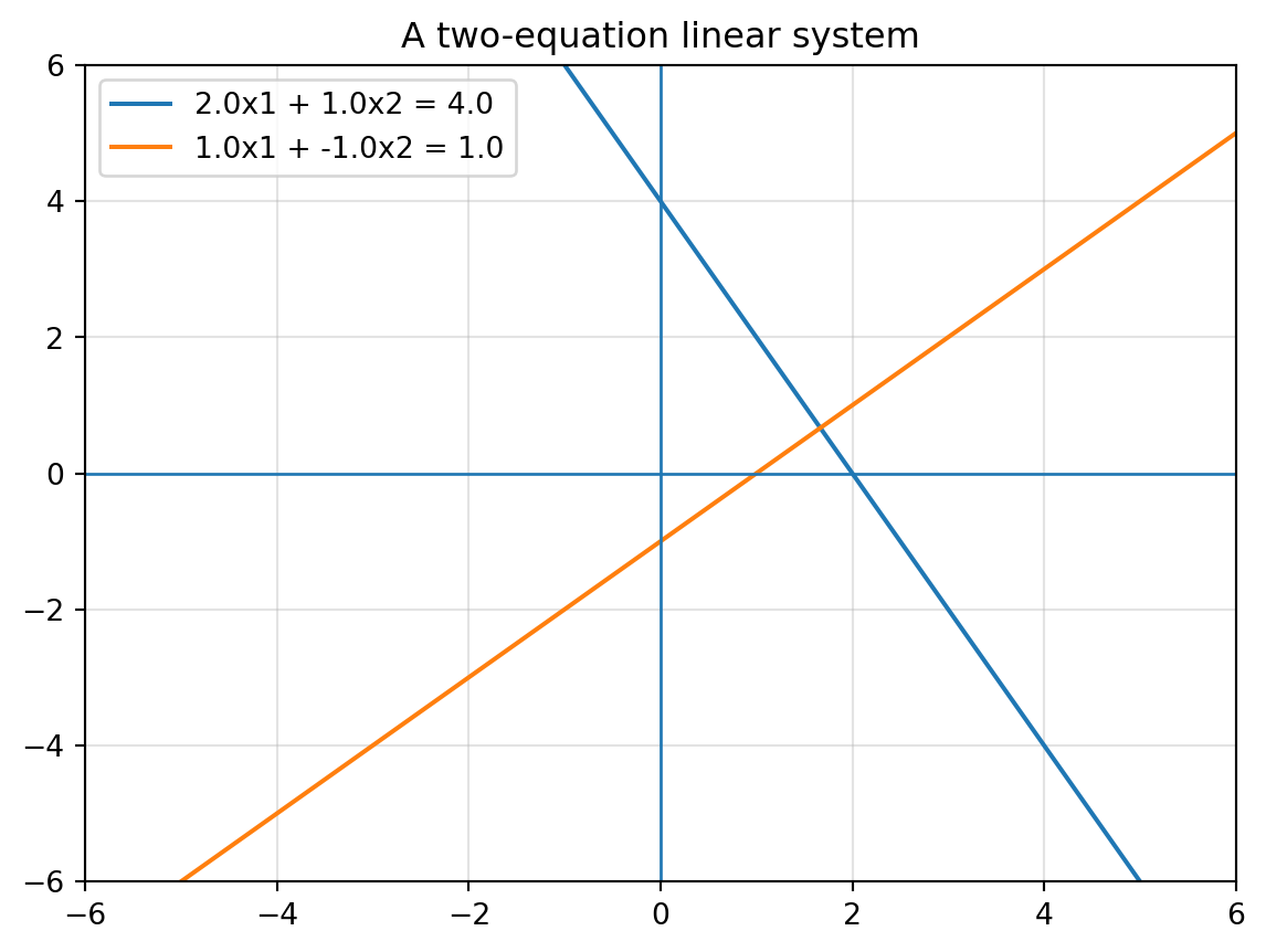
### Exercise 4: Visualize Random Lines
```{python}
def plot_system(a, c, lim=(-6, 6)):
    # a is 2 by 2, c is length 2
    xs = np.linspace(lim[0], lim[1], 400)
    plt.figure(figsize=(7, 5))
    for i in range(2):
        if abs(a[i, 1]) > 1e-12:
            ys = (c[i] - a[i, 0]*xs) / a[i, 1]
            plt.plot(xs, ys, label=f"{a[i,0]:.1f}x1 + {a[i,1]:.1f}x2 = {c[i]:.1f}")
        else:
            plt.axvline(c[i] / a[i, 0], label=f"{a[i,0]:.1f}x1 = {c[i]:.1f}")
    plt.axhline(0, linewidth=1)
    plt.axvline(0, linewidth=1)
    plt.xlim(lim)
    plt.ylim(lim)
    plt.grid(True, alpha=0.35)
    plt.legend()
    plt.title("A two-equation linear system")
    plt.show()

A = np.array([[2, 1], [1, -1]], dtype=float)
b = np.array([4, 1], dtype=float)
plot_system(A, b)
```
### Exercise 5: High-Dimensional Recovery
```{python}
np.random.seed(12)

n = 150
A = np.random.randn(n, n)
x_true = np.random.randn(n)
b = A @ x_true

x_hat = np.linalg.solve(A, b)

print("relative error:", np.linalg.norm(x_hat - x_true) / np.linalg.norm(x_true))
print("relative residual:", np.linalg.norm(A @ x_hat - b) / np.linalg.norm(b))
```
## 7.28 AI Companion Activities
### Activity 1: Explain the Metaphor
Ask an AI tool:
> Explain solving $Ax=b$ as running a matrix machine backwards. Use a real-world analogy different from a smoothie machine.
Then improve the explanation in your own words.
### Activity 2: Diagnose Three Systems
Ask:
> Give me three $2\times 2$ linear systems: one with a unique solution, one with no solution, and one with infinitely many solutions. Explain using both equations and geometry.
Then verify the examples by hand.
### Activity 3: Column Recipe
Ask:
> Explain the column picture of $Ax=b$ using recipes and span.
Then create a new example where two columns build a target vector.
### Activity 4: Numerical Thinking
Ask:
> Why can solving a linear system on a computer produce small numerical errors even when the mathematical solution is exact?
Write a short summary of the difference between exact mathematics and floating-point computation.
## 7.29 Reflection Questions
1. What is the difference between the forward problem and the backward problem?
2. Why does $Ax=b$ represent a system of equations?
3. What does the solution vector $x$ mean in the machine view?
4. What does the solution vector $x$ mean in the column view?
5. Why do row operations preserve solutions?
6. What is a pivot?
7. What does it mean for a system to be consistent?
8. What does it mean for $b$ to be reachable?
9. Why can a singular matrix lead to either no solution or infinitely many solutions?
10. Why is `np.linalg.solve` not a substitute for mathematical understanding?
## 7.30 Chapter Closing
In this chapter, we learned how to solve backwards.
A matrix machine sends an input vector $x$ to an output vector $b$. Solving
$$
Ax=b
$$
means finding the input that produced the output.
We saw the same idea from several angles:
- systems of equations,
- intersections of lines,
- elimination and row operations,
- column combinations,
- reachability,
- information loss,
- and computational solving.
Sometimes the backward problem has one answer. Sometimes it has no answer. Sometimes it has infinitely many answers.
Those cases are not technical details. They reveal whether the matrix machine preserves information, loses information, or asks for an unreachable output.
In the next chapter, we study this question directly:
> When is information lost?
That question leads to rank, null space, column space, and the deeper structure of linear maps.