Local patterns, jumps, and the multiscale language of change
20.1 Opening story: when the important thing happens in one place
In the previous chapter, Fourier analysis gave us a beautiful idea: a signal can be rewritten as a mixture of waves.
That is powerful because waves are excellent at describing rhythm, frequency, and periodic behavior. A musical note, a heartbeat, a vibration, a repeating seasonal pattern, or a smooth oscillation all feel natural in Fourier language.
But not every signal is mainly about rhythm.
Sometimes the most important information is local.
A medical image may contain a sharp boundary between tissue types. A photograph may contain the edge of a face. A financial time series may contain a sudden jump. A sensor signal may be mostly quiet, except for one short burst. A handwritten digit may be recognized by where dark pixels suddenly change to light pixels.
A global wave spreads across the whole signal. An edge lives in one place.
So we need a second language.
Fourier asks:
Which frequencies are present?
Haar wavelets ask:
Where does the signal change, and at what scale?
The central idea of this chapter is:
A Haar wavelet transform rewrites a signal using averages and differences at multiple scales.
This is one of the simplest examples of a multiscale transform. It is also one of the clearest examples of how linear algebra becomes a way of seeing.
20.2 Learning goals
By the end of this chapter, you should be able to:
Explain the difference between global wave features and local wavelet features.
Compute the Haar transform for signals of length \(2\), \(4\), and \(8\).
Interpret Haar coefficients as averages and differences.
Build Haar basis vectors and understand why they are orthonormal.
Use Haar coefficients for compression and denoising.
Compare Fourier and Haar representations for smooth signals and signals with jumps.
Apply one-dimensional Haar ideas to rows, columns, and images.
Use Python to visualize multiscale decomposition.
Connect Haar wavelets to feature extraction, image processing, and AI-era representations.
20.3 1. The smallest Haar transform
The whole story begins with two numbers.
Suppose a signal has only two values:
\[
x = \begin{bmatrix} a \\ b \end{bmatrix}.
\]
Instead of storing \(a\) and \(b\) directly, we can store:
their average-like part,
their difference-like part.
The normalized Haar transform uses
\[
s = \frac{a+b}{\sqrt{2}}, \qquad d = \frac{a-b}{\sqrt{2}}.
\]
The number \(s\) measures the shared level of the two entries. The number \(d\) measures how much the first entry differs from the second.
In matrix form,
\[
\begin{bmatrix} s \\ d \end{bmatrix}
=
\frac{1}{\sqrt{2}}
\begin{bmatrix}
1 & 1 \\
1 & -1
\end{bmatrix}
\begin{bmatrix} a \\ b \end{bmatrix}.
\]
The first row listens for the average. The second row listens for a jump.
20.3.1 Example 1: two neighboring pixels
Suppose two neighboring pixels have brightness values \(80\) and \(84\). Then
\[
s = \frac{80+84}{\sqrt{2}} \approx 115.97,
\qquad
d = \frac{80-84}{\sqrt{2}} \approx -2.83.
\]
The difference coefficient is small, so the two pixels are similar.
Now suppose the values are \(20\) and \(220\). Then
\[
s = \frac{20+220}{\sqrt{2}} \approx 169.71,
\qquad
d = \frac{20-220}{\sqrt{2}} \approx -141.42.
\]
The difference coefficient is large, so there is a strong local edge.
The Haar transform turns local contrast into a coordinate.
20.4 2. Why normalization matters
The factors \(1/\sqrt{2}\) may look like an annoying detail, but they are important. They make the rows of \(H_2\) unit vectors and make the rows orthogonal:
That is a major advantage. The transform changes coordinates, but it does not distort length. It gives a new language for the same signal.
20.5 3. Reconstructing the original signal
Because \(H_2\) is orthogonal, its inverse is its transpose:
\[
H_2^{-1} = H_2^T = H_2.
\]
Therefore,
\[
x = H_2^T \begin{bmatrix} s \\ d \end{bmatrix}.
\]
Written entry by entry,
\[
a = \frac{s+d}{\sqrt{2}},
\qquad
b = \frac{s-d}{\sqrt{2}}.
\]
The average-like coefficient and difference-like coefficient contain all the information. Nothing is lost unless we choose to discard some coefficients.
\(D\) is the large-scale difference between the first half and second half.
\(d_1\) is the local difference inside the first pair.
\(d_2\) is the local difference inside the second pair.
This is the first moment where the word multiscale becomes visible. Haar does not only ask whether the signal changes. It asks where the signal changes and at what scale.
20.7 5. Haar as a basis
For a signal of length \(4\), one orthonormal Haar basis is:
\[
h_0 = \frac{1}{2}[1,1,1,1],
\]
\[
h_1 = \frac{1}{2}[1,1,-1,-1],
\]
\[
h_2 = \frac{1}{\sqrt{2}}[1,-1,0,0],
\]
\[
h_3 = \frac{1}{\sqrt{2}}[0,0,1,-1].
\]
These four vectors form an orthonormal basis of \(\mathbb{R}^4\). Therefore any signal \(x \in \mathbb{R}^4\) can be written as
\[
x = c_0 h_0 + c_1 h_1 + c_2 h_2 + c_3 h_3.
\]
The coefficients are dot products:
\[
c_i = x \cdot h_i.
\]
This should feel familiar. Fourier coefficients were also projections onto basis vectors. PCA coefficients were also coordinates along special directions. The new idea is the shape of the basis vectors.
Fourier basis vectors oscillate across the whole domain. Haar basis vectors are localized blocks of positive and negative values.
The Haar transform is just a change of orthonormal coordinates. The coordinates have a special interpretation: overall level, coarse contrast, and local detail.
20.9 7. Multiscale thinking
A signal of length \(8\) can be decomposed into:
one global average,
one difference between the two halves,
two differences between quarters,
four differences between neighboring pairs.
The structure looks like a tree:
level 0:  [whole signal average]
level 1:  [left half vs right half]
level 2:  [quarter differences]
level 3:  [pair differences]
This tree is why Haar is useful for local structure. A large coefficient at a fine scale means a local jump. A large coefficient at a coarse scale means a broad contrast between larger regions.
20.9.1 Example 2: one step edge
Consider the signal
\[
x = [1,1,1,1,5,5,5,5]^T.
\]
There is no small-scale oscillation inside each half. But there is a large jump between the first half and second half.
So Haar will produce a large coefficient at the scale comparing halves, and small coefficients at the finest scale.
20.9.2 Example 3: alternating noise
Consider
\[
x = [1,-1,1,-1,1,-1,1,-1]^T.
\]
This signal changes at every step. Its finest-scale Haar coefficients will be large.
Haar separates broad structure from local detail.
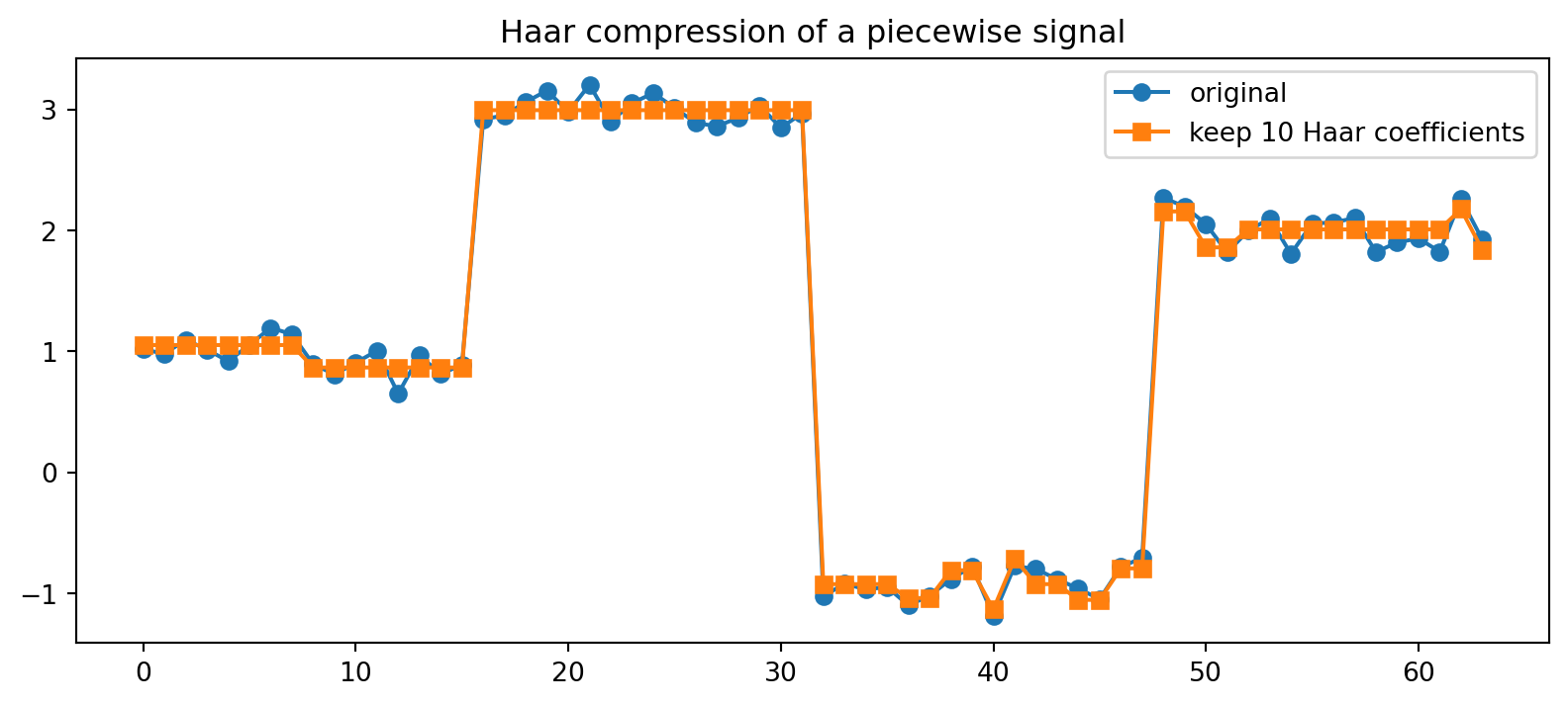
20.10 8. Compression by keeping important coefficients
Suppose a signal has Haar coefficients
\[
c = [c_0,c_1,\dots,c_{n-1}]^T.
\]
If many coefficients are small, we can approximate the signal by keeping only the largest few coefficients.
Let \(\tilde c\) be the vector obtained by setting small coefficients to zero. Then
\[
\tilde x = H^T \tilde c
\]
is a compressed approximation to the original signal.
Because \(H\) is orthogonal, the squared reconstruction error is exactly the energy of the discarded coefficients:
\[
\|x - \tilde x\|^2 = \|c - \tilde c\|^2.
\]
This is a beautiful linear algebra fact. In an orthonormal coordinate system, error can be measured coefficient by coefficient.
20.11 9. Denoising by thresholding
Noise often creates many small coefficients. Meaningful structure often creates fewer larger coefficients.
The idea is not magic. It is geometry. We change coordinates to a basis where local changes are easier to separate from small random fluctuations.
20.12 10. Haar versus Fourier
Fourier and Haar are both orthonormal coordinate systems. Both represent a signal by projection onto basis vectors. Both can compress data if the signal has a simple structure in that basis.
But they are good at different things.
Signal type
Fourier often does well
Haar often does well
Smooth periodic wave
Yes
Sometimes
Repeating rhythm
Yes
Sometimes
Sharp jump
Needs many waves
Often sparse
Local edge
Global representation
Local representation
Piecewise constant signal
Often less sparse
Very sparse
Sudden burst
Spread across frequencies
Localized coefficients
Fourier gives a frequency microscope. Haar gives a location-and-scale microscope.
20.13 11. Images and two-dimensional Haar ideas
A grayscale image is a matrix. To apply Haar ideas to images, we can transform rows and columns.
If \(X\) is an image matrix and \(H\) is a Haar matrix of matching size, a two-dimensional Haar transform has the form
\[
C = H X H^T.
\]
This is exactly the same pattern as a change of basis for matrices.
The coefficients split the image into:
coarse brightness information,
horizontal changes,
vertical changes,
diagonal changes.
Edges often create large Haar coefficients. Smooth regions often need fewer coefficients.
This is one reason wavelet ideas are important in image compression, denoising, and feature extraction.
20.14 12. Haar as a linear algebra story
This chapter is not mainly about memorizing a special transform. It is about seeing a pattern that appears throughout applied mathematics:
Choose a basis that matches the structure of the data.
Project the data onto that basis.
Interpret the coefficients.
Keep, modify, or remove coefficients.
Transform back.
This same story appeared in:
orthogonal projection,
least squares,
PCA,
SVD,
Fourier analysis,
image compression.
Haar gives one of the clearest examples because the basis vectors are simple, local, and visual.
20.15 13. Worked examples
20.15.1 Worked example 1: Haar transform of length 2
The first coefficient measures the shared level. The second measures the difference between the two entries.
20.18.2 Problem 2
Show that the two rows of \(H_2\) are orthonormal.
Solution
Each row has length
\[
\sqrt{\frac12+\frac12}=1.
\]
Their dot product is
\[
\frac12 - \frac12 = 0.
\]
So the rows are orthonormal.
20.18.3 Problem 3
For
\[
x=[3,3,3,3]^T,
\]
what do you expect the Haar coefficients to look like?
Solution
Only the global average coefficient should be nonzero. There are no local differences and no coarse contrast.
Using \(H_4\),
\[
c=[6,0,0,0]^T.
\]
20.18.4 Problem 4
For
\[
x=[1,1,5,5]^T,
\]
which coefficient should be large: a coarse coefficient or a fine coefficient?
Solution
The important change occurs between the first half and second half. So the coarse half-difference coefficient should be large, while the within-pair coefficients should be zero.
20.18.5 Problem 5
Explain why Haar compression works especially well for piecewise constant signals.
Solution
A piecewise constant signal has many regions where neighboring values are equal or nearly equal. Therefore many local difference coefficients are zero or small. Only coefficients near jumps or at important coarse contrasts are large. So the signal can often be represented accurately using relatively few coefficients.
20.19 17. Challenge problems
20.19.1 Challenge 1
Construct the \(8\times 8\) Haar matrix and verify numerically that it is orthogonal.
20.19.2 Challenge 2
Create two signals of length \(64\):
a smooth sine wave,
a piecewise constant step signal.
Compare the number of Fourier coefficients and Haar coefficients needed to approximate each signal well.
20.19.3 Challenge 3
Use Haar thresholding to denoise a noisy step signal. How does the result change as the threshold increases?
20.19.4 Challenge 4
Apply a two-dimensional Haar transform to a small image matrix. Which coefficients correspond to coarse brightness information? Which coefficients respond to edges?
20.20 18. AI companion activities
Use an AI assistant as a study partner, but make it explain rather than merely answer.
Ask: “Explain Haar wavelets to a student who understands projections and orthogonal bases.”
Ask: “Compare Fourier and Haar using one smooth signal and one signal with a jump.”
Ask: “Create a small length-8 Haar transform example with full reconstruction.”
Ask: “Why does thresholding small Haar coefficients denoise a signal?”
Ask: “How is a two-dimensional Haar transform related to image edges?”
20.21 19. Chapter summary
Fourier analysis taught us that signals can be described by global waves. Haar wavelets teach us that signals can also be described by local averages and differences.
The key ideas are:
Haar transforms are orthonormal changes of coordinates.
Haar coefficients measure information at different scales.
Large detail coefficients indicate jumps, edges, or local changes.
Small coefficients can often be discarded for compression or denoising.
Haar is especially useful for piecewise constant or locally structured data.
In two dimensions, Haar ideas help describe image edges and multiscale structure.
The bigger lesson is that a basis is a language. Fourier speaks in waves. PCA speaks in directions of variation. SVD speaks in rank-one layers. Haar speaks in local changes.
Linear algebra lets us move between these languages.
Source Code
---title: "Chapter 20: Haar Wavelets"subtitle: "Local patterns, jumps, and the multiscale language of change"format: html: toc: true toc-depth: 3 number-sections: true code-fold: true code-tools: truejupyter: python3---## Opening story: when the important thing happens in one placeIn the previous chapter, Fourier analysis gave us a beautiful idea:a signal can be rewritten as a mixture of waves.That is powerful because waves are excellent at describing rhythm, frequency, and periodic behavior.A musical note, a heartbeat, a vibration, a repeating seasonal pattern, or a smooth oscillation all feel natural in Fourier language.But not every signal is mainly about rhythm.Sometimes the most important information is local.A medical image may contain a sharp boundary between tissue types.A photograph may contain the edge of a face.A financial time series may contain a sudden jump.A sensor signal may be mostly quiet, except for one short burst.A handwritten digit may be recognized by where dark pixels suddenly change to light pixels.A global wave spreads across the whole signal.An edge lives in one place.So we need a second language.Fourier asks:> Which frequencies are present?Haar wavelets ask:> Where does the signal change, and at what scale?The central idea of this chapter is:> A Haar wavelet transform rewrites a signal using averages and differences at multiple scales.This is one of the simplest examples of a multiscale transform.It is also one of the clearest examples of how linear algebra becomes a way of seeing.## Learning goalsBy the end of this chapter, you should be able to:1. Explain the difference between global wave features and local wavelet features.2. Compute the Haar transform for signals of length $2$, $4$, and $8$.3. Interpret Haar coefficients as averages and differences.4. Build Haar basis vectors and understand why they are orthonormal.5. Use Haar coefficients for compression and denoising.6. Compare Fourier and Haar representations for smooth signals and signals with jumps.7. Apply one-dimensional Haar ideas to rows, columns, and images.8. Use Python to visualize multiscale decomposition.9. Connect Haar wavelets to feature extraction, image processing, and AI-era representations.## 1. The smallest Haar transformThe whole story begins with two numbers.Suppose a signal has only two values:$$x = \begin{bmatrix} a \\ b \end{bmatrix}.$$Instead of storing $a$ and $b$ directly, we can store:- their average-like part,- their difference-like part.The normalized Haar transform uses$$s = \frac{a+b}{\sqrt{2}}, \qquad d = \frac{a-b}{\sqrt{2}}.$$The number $s$ measures the shared level of the two entries.The number $d$ measures how much the first entry differs from the second.In matrix form,$$\begin{bmatrix} s \\ d \end{bmatrix}=\frac{1}{\sqrt{2}}\begin{bmatrix}1 & 1 \\1 & -1\end{bmatrix}\begin{bmatrix} a \\ b \end{bmatrix}.$$Call this matrix $H_2$:$$H_2 = \frac{1}{\sqrt{2}}\begin{bmatrix}1 & 1 \\1 & -1\end{bmatrix}.$$This is the smallest Haar matrix.It has two rows:$$\frac{1}{\sqrt{2}}[1,1]\qquad \text{and} \qquad\frac{1}{\sqrt{2}}[1,-1].$$The first row listens for the average.The second row listens for a jump.### Example 1: two neighboring pixelsSuppose two neighboring pixels have brightness values $80$ and $84$.Then$$s = \frac{80+84}{\sqrt{2}} \approx 115.97,\qquadd = \frac{80-84}{\sqrt{2}} \approx -2.83.$$The difference coefficient is small, so the two pixels are similar.Now suppose the values are $20$ and $220$.Then$$s = \frac{20+220}{\sqrt{2}} \approx 169.71,\qquadd = \frac{20-220}{\sqrt{2}} \approx -141.42.$$The difference coefficient is large, so there is a strong local edge.The Haar transform turns local contrast into a coordinate.## 2. Why normalization mattersThe factors $1/\sqrt{2}$ may look like an annoying detail, but they are important.They make the rows of $H_2$ unit vectors and make the rows orthogonal:$$\frac{1}{\sqrt{2}}[1,1] \cdot \frac{1}{\sqrt{2}}[1,-1]= \frac{1-1}{2} = 0.$$Also,$$\left\|\frac{1}{\sqrt{2}}[1,1]\right\| = 1,\qquad\left\|\frac{1}{\sqrt{2}}[1,-1]\right\| = 1.$$So $H_2$ is an orthogonal matrix:$$H_2^T H_2 = I.$$This means the transform preserves energy:$$\|H_2x\|^2 = \|x\|^2.$$That is a major advantage.The transform changes coordinates, but it does not distort length.It gives a new language for the same signal.## 3. Reconstructing the original signalBecause $H_2$ is orthogonal, its inverse is its transpose:$$H_2^{-1} = H_2^T = H_2.$$Therefore,$$x = H_2^T \begin{bmatrix} s \\ d \end{bmatrix}.$$Written entry by entry,$$a = \frac{s+d}{\sqrt{2}},\qquadb = \frac{s-d}{\sqrt{2}}.$$The average-like coefficient and difference-like coefficient contain all the information.Nothing is lost unless we choose to discard some coefficients.## 4. From two numbers to four numbersNow suppose the signal has four entries:$$x = \begin{bmatrix} x_1 \\ x_2 \\ x_3 \\ x_4 \end{bmatrix}.$$A natural first step is to compare neighboring pairs:$$s_1 = \frac{x_1+x_2}{\sqrt{2}}, \qquad d_1 = \frac{x_1-x_2}{\sqrt{2}},$$$$s_2 = \frac{x_3+x_4}{\sqrt{2}}, \qquad d_2 = \frac{x_3-x_4}{\sqrt{2}}.$$Now we have two coarse averages $s_1,s_2$ and two local differences $d_1,d_2$.But Haar does not stop there.It compares the averages again:$$S = \frac{s_1+s_2}{\sqrt{2}},\qquadD = \frac{s_1-s_2}{\sqrt{2}}.$$The final transform can be organized as:$$\text{Haar coefficients} = [S, D, d_1, d_2]^T.$$Interpretation:- $S$ is the overall average level.- $D$ is the large-scale difference between the first half and second half.- $d_1$ is the local difference inside the first pair.- $d_2$ is the local difference inside the second pair.This is the first moment where the word **multiscale** becomes visible.Haar does not only ask whether the signal changes.It asks where the signal changes and at what scale.## 5. Haar as a basisFor a signal of length $4$, one orthonormal Haar basis is:$$h_0 = \frac{1}{2}[1,1,1,1],$$$$h_1 = \frac{1}{2}[1,1,-1,-1],$$$$h_2 = \frac{1}{\sqrt{2}}[1,-1,0,0],$$$$h_3 = \frac{1}{\sqrt{2}}[0,0,1,-1].$$These four vectors form an orthonormal basis of $\mathbb{R}^4$.Therefore any signal $x \in \mathbb{R}^4$ can be written as$$x = c_0 h_0 + c_1 h_1 + c_2 h_2 + c_3 h_3.$$The coefficients are dot products:$$c_i = x \cdot h_i.$$This should feel familiar.Fourier coefficients were also projections onto basis vectors.PCA coefficients were also coordinates along special directions.The new idea is the shape of the basis vectors.Fourier basis vectors oscillate across the whole domain.Haar basis vectors are localized blocks of positive and negative values.## 6. The matrix viewStack the basis vectors as rows:$$H_4 =\begin{bmatrix}\frac12 & \frac12 & \frac12 & \frac12 \\\frac12 & \frac12 & -\frac12 & -\frac12 \\\frac{1}{\sqrt2} & -\frac{1}{\sqrt2} & 0 & 0 \\0 & 0 & \frac{1}{\sqrt2} & -\frac{1}{\sqrt2}\end{bmatrix}.$$Then the Haar coefficients are$$c = H_4 x.$$Since the rows form an orthonormal basis,$$H_4 H_4^T = I,\qquadH_4^T H_4 = I.$$So reconstruction is$$x = H_4^T c.$$The Haar transform is just a change of orthonormal coordinates.The coordinates have a special interpretation: overall level, coarse contrast, and local detail.## 7. Multiscale thinkingA signal of length $8$ can be decomposed into:- one global average,- one difference between the two halves,- two differences between quarters,- four differences between neighboring pairs.The structure looks like a tree:```textlevel 0: [whole signal average]level 1: [left half vs right half]level 2: [quarter differences]level 3: [pair differences]```This tree is why Haar is useful for local structure.A large coefficient at a fine scale means a local jump.A large coefficient at a coarse scale means a broad contrast between larger regions.### Example 2: one step edgeConsider the signal$$x = [1,1,1,1,5,5,5,5]^T.$$There is no small-scale oscillation inside each half.But there is a large jump between the first half and second half.So Haar will produce a large coefficient at the scale comparing halves, and small coefficients at the finest scale.### Example 3: alternating noiseConsider$$x = [1,-1,1,-1,1,-1,1,-1]^T.$$This signal changes at every step.Its finest-scale Haar coefficients will be large.Haar separates broad structure from local detail.## 8. Compression by keeping important coefficientsSuppose a signal has Haar coefficients$$c = [c_0,c_1,\dots,c_{n-1}]^T.$$If many coefficients are small, we can approximate the signal by keeping only the largest few coefficients.Let $\tilde c$ be the vector obtained by setting small coefficients to zero.Then$$\tilde x = H^T \tilde c$$is a compressed approximation to the original signal.Because $H$ is orthogonal, the squared reconstruction error is exactly the energy of the discarded coefficients:$$\|x - \tilde x\|^2 = \|c - \tilde c\|^2.$$This is a beautiful linear algebra fact.In an orthonormal coordinate system, error can be measured coefficient by coefficient.## 9. Denoising by thresholdingNoise often creates many small coefficients.Meaningful structure often creates fewer larger coefficients.A simple denoising rule is:$$\tilde c_i =\begin{cases}c_i, & |c_i| \ge \tau, \\0, & |c_i| < \tau.\end{cases}$$Then reconstruct$$\tilde x = H^T \tilde c.$$This is called thresholding.The idea is not magic.It is geometry.We change coordinates to a basis where local changes are easier to separate from small random fluctuations.## 10. Haar versus FourierFourier and Haar are both orthonormal coordinate systems.Both represent a signal by projection onto basis vectors.Both can compress data if the signal has a simple structure in that basis.But they are good at different things.| Signal type | Fourier often does well | Haar often does well ||---|---:|---:|| Smooth periodic wave | Yes | Sometimes || Repeating rhythm | Yes | Sometimes || Sharp jump | Needs many waves | Often sparse || Local edge | Global representation | Local representation || Piecewise constant signal | Often less sparse | Very sparse || Sudden burst | Spread across frequencies | Localized coefficients |Fourier gives a frequency microscope.Haar gives a location-and-scale microscope.## 11. Images and two-dimensional Haar ideasA grayscale image is a matrix.To apply Haar ideas to images, we can transform rows and columns.If $X$ is an image matrix and $H$ is a Haar matrix of matching size, a two-dimensional Haar transform has the form$$C = H X H^T.$$This is exactly the same pattern as a change of basis for matrices.The coefficients split the image into:- coarse brightness information,- horizontal changes,- vertical changes,- diagonal changes.Edges often create large Haar coefficients.Smooth regions often need fewer coefficients.This is one reason wavelet ideas are important in image compression, denoising, and feature extraction.## 12. Haar as a linear algebra storyThis chapter is not mainly about memorizing a special transform.It is about seeing a pattern that appears throughout applied mathematics:1. Choose a basis that matches the structure of the data.2. Project the data onto that basis.3. Interpret the coefficients.4. Keep, modify, or remove coefficients.5. Transform back.This same story appeared in:- orthogonal projection,- least squares,- PCA,- SVD,- Fourier analysis,- image compression.Haar gives one of the clearest examples because the basis vectors are simple, local, and visual.## 13. Worked examples### Worked example 1: Haar transform of length 2Let$$x = \begin{bmatrix} 6 \\ 2 \end{bmatrix}.$$Then$$H_2x = \frac{1}{\sqrt2}\begin{bmatrix}1 & 1 \\1 & -1\end{bmatrix}\begin{bmatrix} 6 \\ 2 \end{bmatrix}=\begin{bmatrix}8/\sqrt2 \\4/\sqrt2\end{bmatrix}=\begin{bmatrix}4\sqrt2 \\2\sqrt2\end{bmatrix}.$$The average-like coefficient is $4\sqrt2$.The difference-like coefficient is $2\sqrt2$.### Worked example 2: length 4 decompositionLet$$x = [4,4,8,8]^T.$$Using the $H_4$ basis above,$$c_0 = x\cdot h_0 = 12,$$$$c_1 = x\cdot h_1 = -4,$$$$c_2 = x\cdot h_2 = 0,$$$$c_3 = x\cdot h_3 = 0.$$The signal has no local pair differences.Its structure is entirely global average plus a coarse left-right contrast.### Worked example 3: local jumpLet$$x = [4,8,4,8]^T.$$Then the coarse half difference is small, but the within-pair differences are large.This signal has fine-scale changes.The Haar coefficients identify the scale at which the change occurs.## 14. Python: build Haar matrices```{python}import numpy as npdef haar_matrix(n):"""Return an orthonormal Haar matrix for n = 2^m."""if n ==1:return np.array([[1.0]]) H_small = haar_matrix(n //2) top = np.kron(H_small, [1, 1]) / np.sqrt(2) bottom = np.kron(np.eye(n //2), [1, -1]) / np.sqrt(2)return np.vstack([top, bottom])H8 = haar_matrix(8)print(np.round(H8, 3))print("Orthogonality check:", np.round(np.linalg.norm(H8 @ H8.T - np.eye(8)), 12))```## 15. Python: transform, compress, reconstruct```{python}import matplotlib.pyplot as pltn =64x = np.r_[np.ones(16), 3*np.ones(16), -1*np.ones(16), 2*np.ones(16)]x = x +0.15*np.random.default_rng(0).normal(size=n)H = haar_matrix(n)c = H @ x# Keep the 10 largest coefficients in magnitudek =10idx = np.argsort(np.abs(c))[-k:]c_keep = np.zeros_like(c)c_keep[idx] = c[idx]x_hat = H.T @ c_keepplt.figure(figsize=(10, 4))plt.plot(x, marker='o', label='original')plt.plot(x_hat, marker='s', label=f'keep {k} Haar coefficients')plt.legend()plt.title('Haar compression of a piecewise signal')plt.show()```## 16. Practice problems### Problem 1Compute the Haar transform of$$x = [10, 6]^T.$$Interpret the two coefficients.<details><summary>Solution</summary>$$H_2x = \frac{1}{\sqrt2}[16,4]^T = [8\sqrt2,2\sqrt2]^T.$$The first coefficient measures the shared level.The second measures the difference between the two entries.</details>### Problem 2Show that the two rows of $H_2$ are orthonormal.<details><summary>Solution</summary>Each row has length$$\sqrt{\frac12+\frac12}=1.$$Their dot product is$$\frac12 - \frac12 = 0.$$So the rows are orthonormal.</details>### Problem 3For$$x=[3,3,3,3]^T,$$what do you expect the Haar coefficients to look like?<details><summary>Solution</summary>Only the global average coefficient should be nonzero.There are no local differences and no coarse contrast.Using $H_4$,$$c=[6,0,0,0]^T.$$</details>### Problem 4For$$x=[1,1,5,5]^T,$$which coefficient should be large: a coarse coefficient or a fine coefficient?<details><summary>Solution</summary>The important change occurs between the first half and second half.So the coarse half-difference coefficient should be large, while the within-pair coefficients should be zero.</details>### Problem 5Explain why Haar compression works especially well for piecewise constant signals.<details><summary>Solution</summary>A piecewise constant signal has many regions where neighboring values are equal or nearly equal.Therefore many local difference coefficients are zero or small.Only coefficients near jumps or at important coarse contrasts are large.So the signal can often be represented accurately using relatively few coefficients.</details>## 17. Challenge problems### Challenge 1Construct the $8\times 8$ Haar matrix and verify numerically that it is orthogonal.### Challenge 2Create two signals of length $64$:1. a smooth sine wave,2. a piecewise constant step signal.Compare the number of Fourier coefficients and Haar coefficients needed to approximate each signal well.### Challenge 3Use Haar thresholding to denoise a noisy step signal.How does the result change as the threshold increases?### Challenge 4Apply a two-dimensional Haar transform to a small image matrix.Which coefficients correspond to coarse brightness information?Which coefficients respond to edges?## 18. AI companion activitiesUse an AI assistant as a study partner, but make it explain rather than merely answer.1. Ask: "Explain Haar wavelets to a student who understands projections and orthogonal bases."2. Ask: "Compare Fourier and Haar using one smooth signal and one signal with a jump."3. Ask: "Create a small length-8 Haar transform example with full reconstruction."4. Ask: "Why does thresholding small Haar coefficients denoise a signal?"5. Ask: "How is a two-dimensional Haar transform related to image edges?"## 19. Chapter summaryFourier analysis taught us that signals can be described by global waves.Haar wavelets teach us that signals can also be described by local averages and differences.The key ideas are:- Haar transforms are orthonormal changes of coordinates.- Haar coefficients measure information at different scales.- Large detail coefficients indicate jumps, edges, or local changes.- Small coefficients can often be discarded for compression or denoising.- Haar is especially useful for piecewise constant or locally structured data.- In two dimensions, Haar ideas help describe image edges and multiscale structure.The bigger lesson is that a basis is a language.Fourier speaks in waves.PCA speaks in directions of variation.SVD speaks in rank-one layers.Haar speaks in local changes.Linear algebra lets us move between these languages.