---
title: "Chapter 19: Fourier"
subtitle: "Learning to hear the hidden coordinates of a signal"
format:
html:
toc: true
toc-depth: 3
number-sections: true
code-fold: true
code-tools: true
jupyter: python3
---
## Opening story: one sound, many hidden notes
A piano chord reaches your ear as one sound.
A microphone does not record the names of the notes. It records a long list of numbers: air pressure measured again and again over time.
To the computer, the chord is a vector.
But that vector is not random. Hidden inside it are waves. Some waves are slow and deep. Some are fast and bright. Some are strong. Some are barely present. Fourier analysis is the art of discovering these hidden waves.
The main idea of this chapter is simple and powerful:
::: {.callout-important}
## Central idea
A signal can be described in two languages:
- the **time language**, which says what the signal does at each time;
- the **frequency language**, which says how much of each wave is inside the signal.
Fourier analysis is a change of coordinates from time to frequency.
:::
This chapter continues the story of linear algebra. We have already learned about vectors, bases, orthogonality, projection, SVD, and PCA. Fourier analysis brings all of these ideas into one beautiful setting:
> A Fourier transform is a coordinate change onto an orthogonal wave basis.
That sentence is the whole chapter in miniature.
## Learning goals
By the end of this chapter, you should be able to:
1. Treat a finite signal as a vector in $\mathbb{R}^n$ or $\mathbb{C}^n$.
2. Explain sine and cosine waves as basis patterns.
3. Interpret amplitude, frequency, and phase.
4. Compute Fourier coefficients as projections onto wave directions.
5. Understand why orthogonality makes Fourier decomposition clean.
6. Use the discrete Fourier transform (DFT) and fast Fourier transform (FFT) in Python.
7. Build simple filters for denoising and smoothing.
8. Use Fourier coefficients for compression.
9. Connect Fourier ideas to images, data science, and machine learning.
## 19.1 A signal is a vector
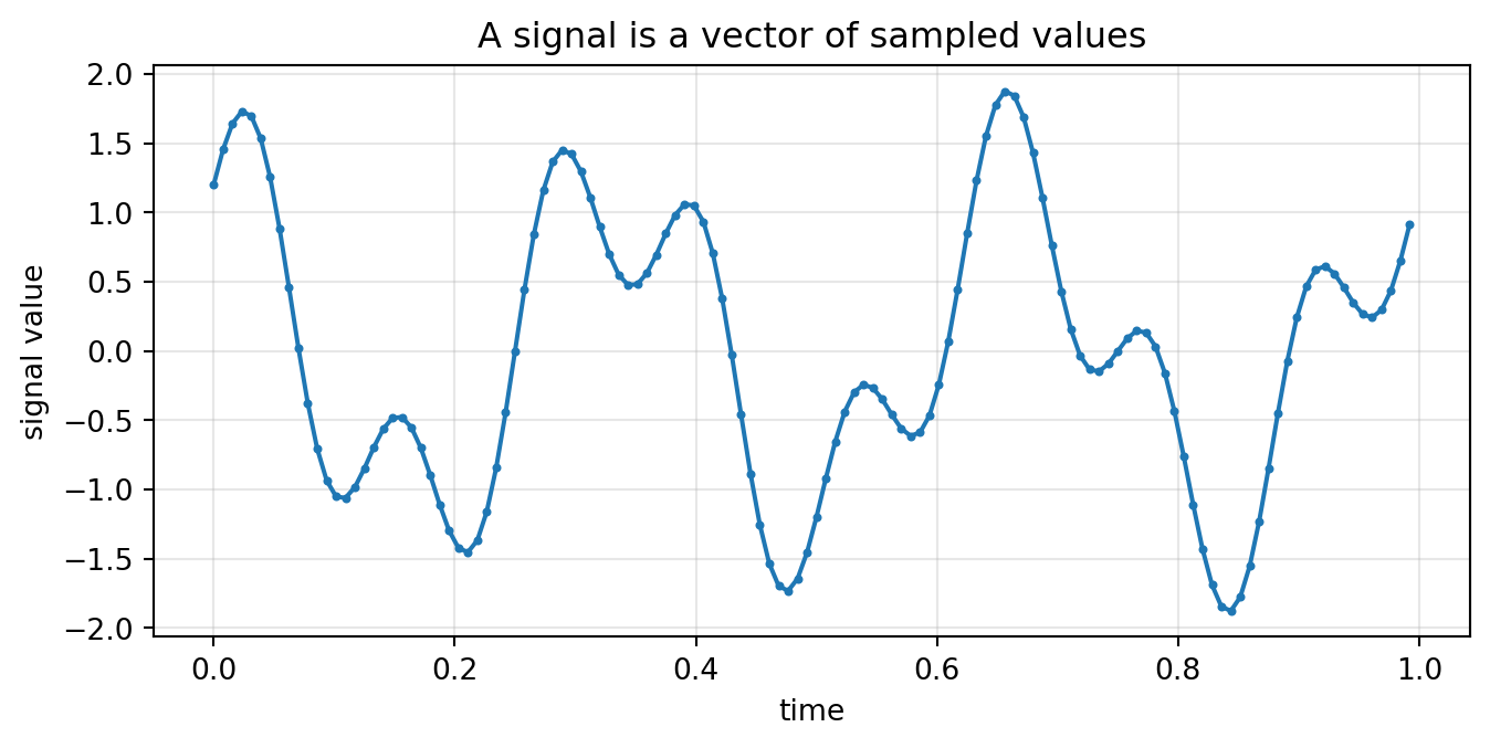
A **signal** is any quantity that changes over time, space, or position. Examples include sound pressure, brightness along an image row, temperature over days, voltage over time, and heart rate measured every second.
If we measure a signal at $n$ equally spaced times, we obtain a vector
$$
x = \begin{bmatrix}
x_0 \\
x_1 \\
\vdots \\
x_{n-1}
\end{bmatrix}.
$$
The coordinate $x_j$ is the value of the signal at the $j$th sample.
::: {.callout-note}
## Signal-as-vector viewpoint
A finite signal is a vector. Therefore we can add signals, scale signals, measure distances between signals, compute dot products, project signals onto subspaces, and change bases.
:::
```{python}
import numpy as np
import matplotlib.pyplot as plt

n = 128
t = np.linspace(0, 1, n, endpoint=False)
x = 1.2*np.cos(2*np.pi*3*t) + 0.7*np.sin(2*np.pi*8*t)

plt.figure(figsize=(8, 3.5))
plt.plot(t, x, marker='o', markersize=2)
plt.xlabel('time')
plt.ylabel('signal value')
plt.title('A signal is a vector of sampled values')
plt.grid(True, alpha=0.3)
plt.show()
```
The plot looks continuous because we connect the dots, but the computer stores the signal as a finite vector.
## 19.2 Waves as building blocks
Fourier analysis uses wave patterns as building blocks. The most familiar waves are
$$
\cos(2\pi f t)
\qquad \text{and} \qquad
\sin(2\pi f t),
$$
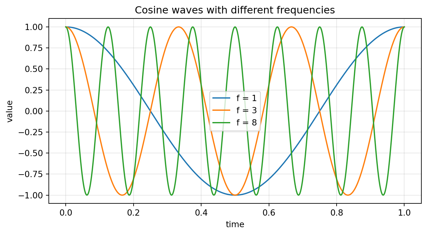
where $f$ is the **frequency**. Frequency counts how many cycles the wave completes per unit time.
A wave with a larger frequency oscillates faster.
```{python}
t = np.linspace(0, 1, 500)
plt.figure(figsize=(8, 4))
for f in [1, 3, 8]:
    plt.plot(t, np.cos(2*np.pi*f*t), label=f'f = {f}')
plt.xlabel('time')
plt.ylabel('value')
plt.title('Cosine waves with different frequencies')
plt.legend()
plt.grid(True, alpha=0.3)
plt.show()
```
A single wave is simple. A sum of waves can be rich.
$$
x(t) = 1.5\cos(2\pi \cdot 2t) + 0.7\sin(2\pi \cdot 7t) + 0.3\cos(2\pi \cdot 15t).
$$
In linear algebra language, this is a **linear combination** of wave vectors.
## 19.3 Amplitude, frequency, and phase
A general cosine wave can be written as
$$
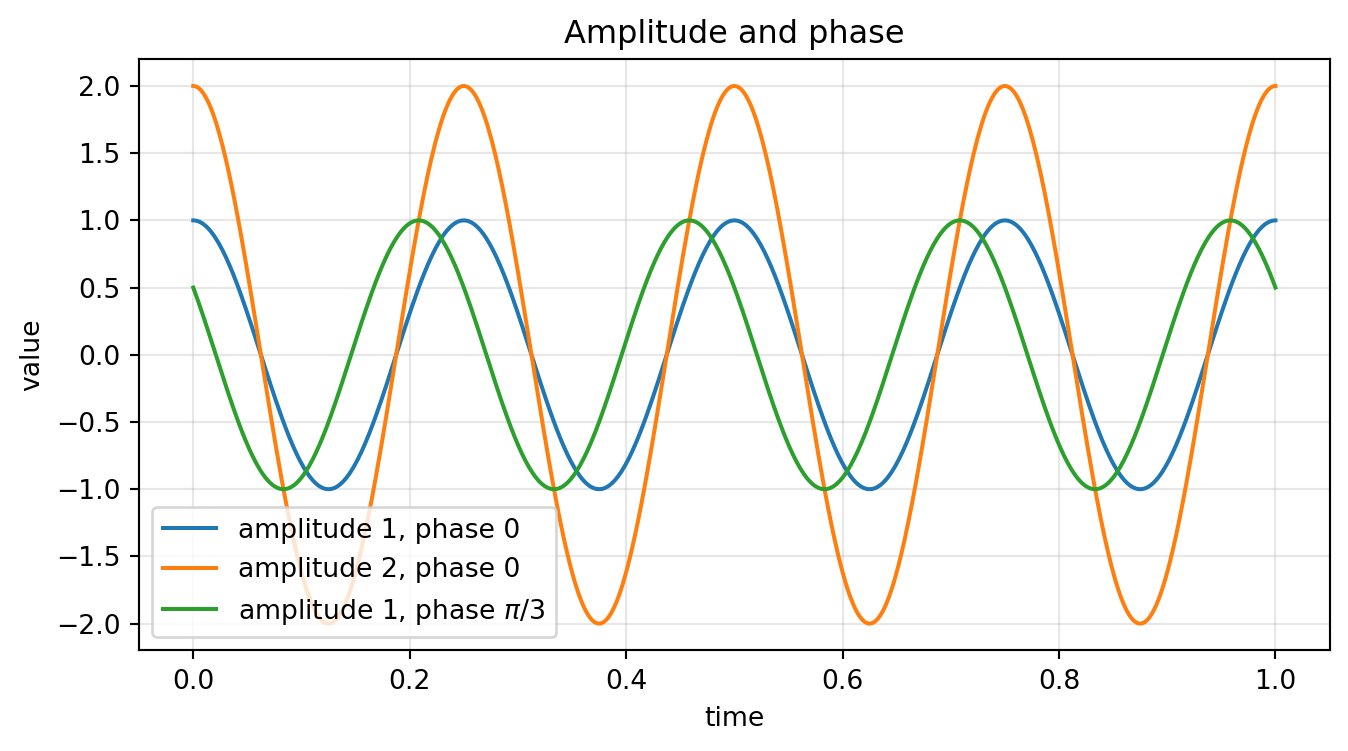
A\cos(2\pi f t + \phi).
$$
Here:
- $A$ is the **amplitude**, controlling height;
- $f$ is the **frequency**, controlling speed of oscillation;
- $\phi$ is the **phase**, controlling horizontal shift.
```{python}
t = np.linspace(0, 1, 600)
plt.figure(figsize=(8, 4))
plt.plot(t, np.cos(2*np.pi*4*t), label='amplitude 1, phase 0')
plt.plot(t, 2*np.cos(2*np.pi*4*t), label='amplitude 2, phase 0')
plt.plot(t, np.cos(2*np.pi*4*t + np.pi/3), label='amplitude 1, phase $\\pi/3$')
plt.xlabel('time')
plt.ylabel('value')
plt.title('Amplitude and phase')
plt.legend()
plt.grid(True, alpha=0.3)
plt.show()
```
Fourier analysis asks: when a complicated signal is given, which amplitudes and phases are hidden inside it?
## 19.4 Orthogonality of waves
The reason Fourier analysis works so cleanly is orthogonality.
For sampled signals $u,v \in \mathbb{R}^n$, the dot product is
$$
u \cdot v = \sum_{j=0}^{n-1} u_j v_j.
$$
Two signals are orthogonal if their dot product is zero. Orthogonal signals do not overlap in the dot-product sense.
For many equally sampled wave patterns, different frequencies are orthogonal.
```{python}
n = 128
j = np.arange(n)
wave3 = np.cos(2*np.pi*3*j/n)
wave8 = np.cos(2*np.pi*8*j/n)

print('dot product between frequency 3 and frequency 8:', np.dot(wave3, wave8).round(10))
print('dot product of frequency 3 with itself:', np.dot(wave3, wave3).round(10))
```
This is the same geometric idea from orthogonal projection. If a signal has some amount of frequency $3$, we can measure it by projecting the signal onto the frequency-$3$ wave direction.
::: {.callout-tip}
## Fourier coefficient as projection
A Fourier coefficient measures how much a signal points in a wave direction.
This is the same idea as finding the coordinate of a vector along an orthogonal basis vector.
:::
## 19.5 Projection onto sine and cosine waves
Suppose $x$ is a sampled signal and $c_k$ is a cosine wave of frequency $k$:
$$
(c_k)_j = \cos\left(\frac{2\pi k j}{n}\right).
$$
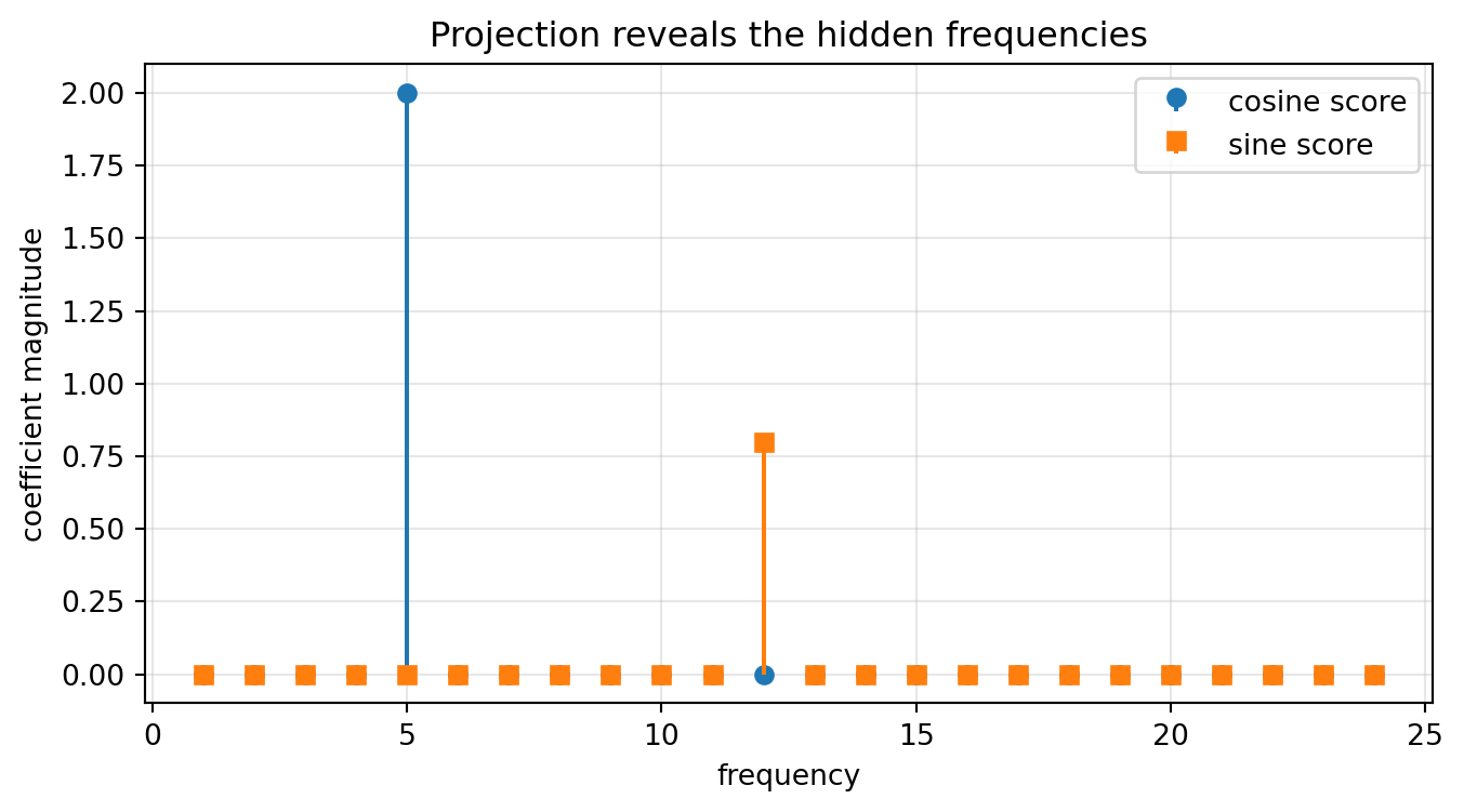
The projection coefficient of $x$ onto $c_k$ is proportional to
$$
x \cdot c_k.
$$
Similarly, if
$$
(s_k)_j = \sin\left(\frac{2\pi k j}{n}\right),
$$
then $x \cdot s_k$ measures how much sine wave of frequency $k$ is present.
```{python}
n = 256
j = np.arange(n)
t = j/n
x = 2.0*np.cos(2*np.pi*5*t) + 0.8*np.sin(2*np.pi*12*t)

cos_scores = []
sin_scores = []
for k in range(1, 25):
    ck = np.cos(2*np.pi*k*j/n)
    sk = np.sin(2*np.pi*k*j/n)
    cos_scores.append(2*np.dot(x, ck)/n)
    sin_scores.append(2*np.dot(x, sk)/n)

plt.figure(figsize=(8, 4))
plt.stem(range(1,25), np.abs(cos_scores), linefmt='C0-', markerfmt='C0o', basefmt=' ', label='cosine score')
plt.stem(range(1,25), np.abs(sin_scores), linefmt='C1-', markerfmt='C1s', basefmt=' ', label='sine score')
plt.xlabel('frequency')
plt.ylabel('coefficient magnitude')
plt.title('Projection reveals the hidden frequencies')
plt.legend()
plt.grid(True, alpha=0.3)
plt.show()
```
The spikes reveal the hidden frequencies.
## 19.6 Complex waves and the DFT
Using sine and cosine separately is useful, but the cleanest notation uses complex numbers. Euler's formula says
$$
e^{i\theta} = \cos \theta + i\sin \theta.
$$
A complex wave of frequency $k$ is
$$
w_k(j) = e^{2\pi i k j/n}.
$$
The **discrete Fourier transform** of a signal $x = (x_0,\ldots,x_{n-1})$ is the list of coefficients
$$
\widehat{x}_k = \sum_{j=0}^{n-1} x_j e^{-2\pi i k j/n},
\qquad k=0,1,\ldots,n-1.
$$
The inverse transform reconstructs the signal:
$$
x_j = \frac{1}{n}\sum_{k=0}^{n-1} \widehat{x}_k e^{2\pi i k j/n}.
$$
::: {.callout-important}
## DFT as a matrix multiplication
The DFT is multiplication by a special matrix $F$ whose entries are complex waves:
$$
F_{k j} = e^{-2\pi i k j/n}.
$$
Thus
$$
\widehat{x} = Fx.
$$
Fourier analysis is linear algebra.
:::
```{python}
n = 8
j = np.arange(n)
k = j.reshape((n,1))
F = np.exp(-2j*np.pi*k*j/n)
np.set_printoptions(precision=2, suppress=True)
print(F)
```
The matrix may look mysterious at first, but each row is a wave pattern used to test the signal.
## 19.7 FFT in Python
The DFT can be computed directly by matrix multiplication, but for large signals this is slow. The **fast Fourier transform** (FFT) is an efficient algorithm for computing the DFT.
In Python, we use `np.fft.fft`.
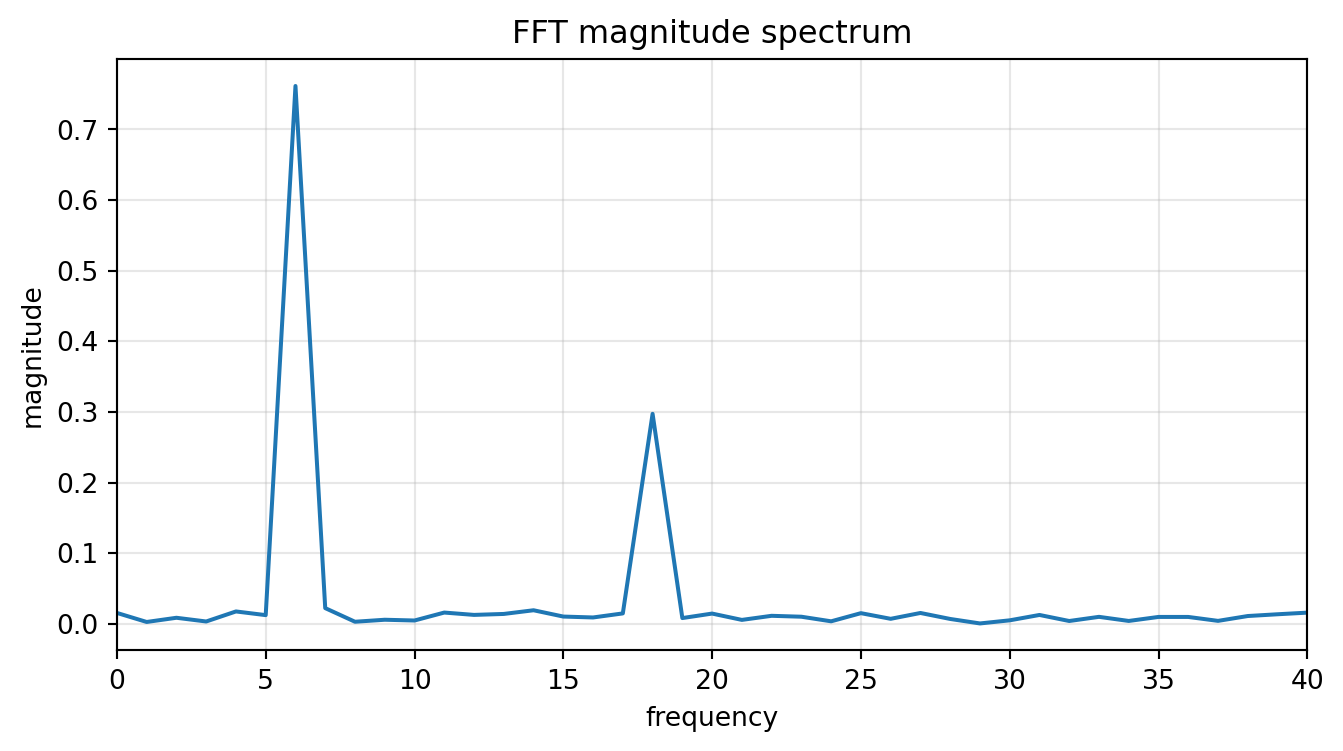
```{python}
n = 512
t = np.linspace(0, 1, n, endpoint=False)
x = 1.5*np.cos(2*np.pi*6*t) + 0.6*np.sin(2*np.pi*18*t) + 0.25*np.random.default_rng(3).normal(size=n)

X = np.fft.fft(x)
freq = np.fft.fftfreq(n, d=1/n)

positive = freq >= 0
plt.figure(figsize=(8, 4))
plt.plot(freq[positive], np.abs(X[positive])/n)
plt.xlim(0, 40)
plt.xlabel('frequency')
plt.ylabel('magnitude')
plt.title('FFT magnitude spectrum')
plt.grid(True, alpha=0.3)
plt.show()
```
Large peaks tell us which frequencies dominate the signal.
## 19.8 Filtering: keeping what we want
Once a signal is written in frequency coordinates, we can edit the signal by editing its Fourier coefficients.
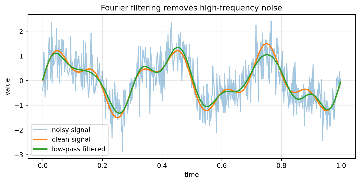
A **low-pass filter** keeps low frequencies and removes high frequencies. This is useful for smoothing noisy signals.
A **high-pass filter** keeps high frequencies and removes low frequencies. This can emphasize sharp changes.
```{python}
rng = np.random.default_rng(4)
n = 512
t = np.linspace(0, 1, n, endpoint=False)
clean = np.sin(2*np.pi*3*t) + 0.5*np.sin(2*np.pi*7*t)
noisy = clean + 0.6*rng.normal(size=n)

Y = np.fft.fft(noisy)
freq = np.fft.fftfreq(n, d=1/n)
mask = np.abs(freq) <= 10
Y_filtered = Y * mask
filtered = np.fft.ifft(Y_filtered).real

plt.figure(figsize=(9, 4))
plt.plot(t, noisy, alpha=0.4, label='noisy signal')
plt.plot(t, clean, linewidth=2, label='clean signal')
plt.plot(t, filtered, linewidth=2, label='low-pass filtered')
plt.xlabel('time')
plt.ylabel('value')
plt.title('Fourier filtering removes high-frequency noise')
plt.legend()
plt.grid(True, alpha=0.3)
plt.show()
```
Filtering is one of the clearest examples of why a change of basis matters. In time coordinates, noise is mixed throughout the signal. In frequency coordinates, some noise may be separated from the meaningful low-frequency structure.
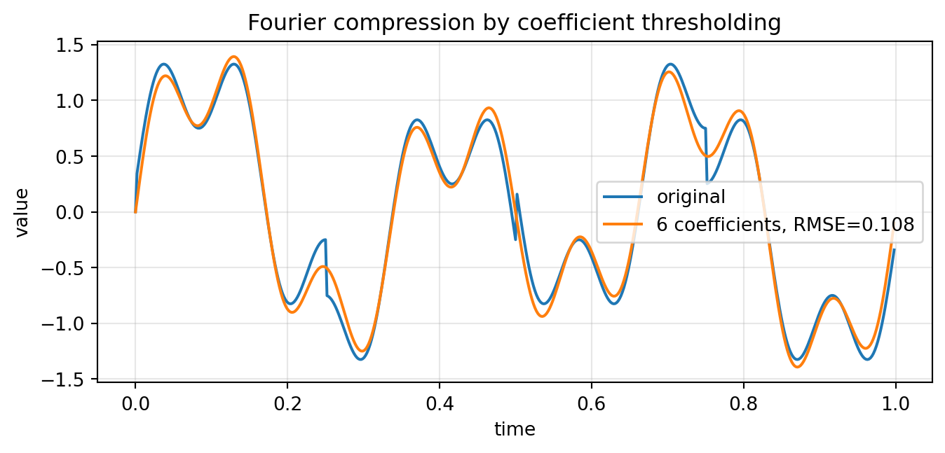
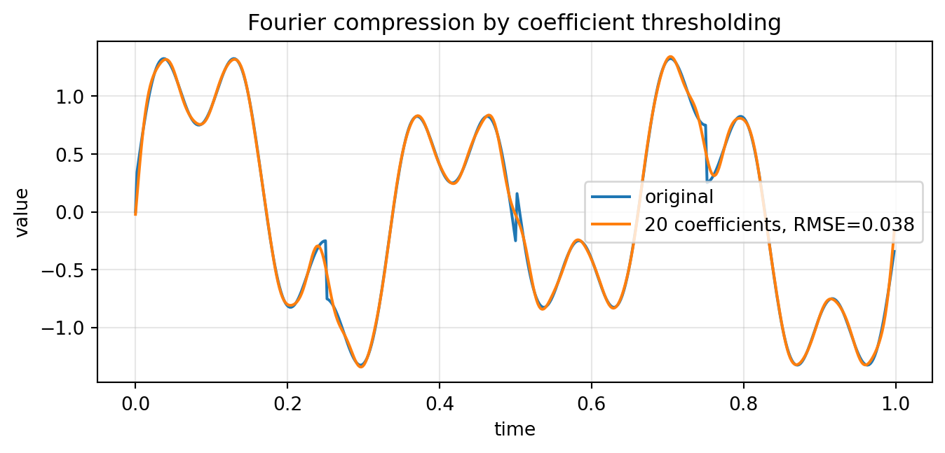
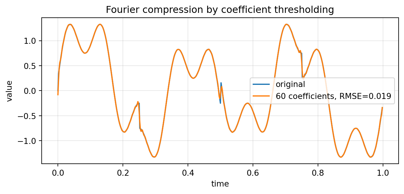
## 19.9 Compression: keeping the largest coefficients
Fourier compression uses a simple idea:
1. Transform the signal into frequency coordinates.
2. Keep only the most important coefficients.
3. Set the rest to zero.
4. Transform back.
This is a projection onto a smaller set of frequency directions.
```{python}
n = 512
t = np.linspace(0, 1, n, endpoint=False)
x = np.sin(2*np.pi*3*t) + 0.5*np.sin(2*np.pi*9*t) + 0.25*np.sign(np.sin(2*np.pi*2*t))
X = np.fft.fft(x)

for keep in [6, 20, 60]:
    idx = np.argsort(np.abs(X))[-keep:]
    Xk = np.zeros_like(X)
    Xk[idx] = X[idx]
    xk = np.fft.ifft(Xk).real
    rmse = np.sqrt(np.mean((x - xk)**2))
    plt.figure(figsize=(8, 3.3))
    plt.plot(t, x, label='original')
    plt.plot(t, xk, label=f'{keep} coefficients, RMSE={rmse:.3f}')
    plt.title('Fourier compression by coefficient thresholding')
    plt.xlabel('time')
    plt.ylabel('value')
    plt.legend()
    plt.grid(True, alpha=0.3)
    plt.show()
```
Smooth signals often compress very well because only a few low frequencies carry most of the information.
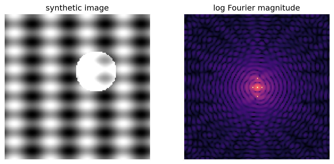
## 19.10 Fourier ideas in images
A grayscale image is a matrix. Each row and column contains spatial variation. Fourier analysis can be extended to two dimensions. The two-dimensional Fourier transform describes an image in terms of horizontal and vertical frequencies.
Low spatial frequencies describe smooth background structure. High spatial frequencies describe edges, fine textures, and noise.
```{python}
# Synthetic image with smooth and sharp structures
m = 128
y, xgrid = np.mgrid[0:m, 0:m]
img = 0.5 + 0.3*np.sin(2*np.pi*xgrid/32) + 0.2*np.cos(2*np.pi*y/16)
img += (((xgrid-80)**2 + (y-50)**2) < 18**2)*0.6
img = np.clip(img, 0, 1)

F2 = np.fft.fftshift(np.fft.fft2(img))
mag = np.log1p(np.abs(F2))

fig, ax = plt.subplots(1, 2, figsize=(9, 4))
ax[0].imshow(img, cmap='gray')
ax[0].set_title('synthetic image')
ax[0].axis('off')
ax[1].imshow(mag, cmap='magma')
ax[1].set_title('log Fourier magnitude')
ax[1].axis('off')
plt.show()
```
This is the basis of many methods in image processing: smoothing, sharpening, compression, denoising, and texture analysis.
## 19.11 Fourier, PCA, and SVD: three coordinate stories
Fourier, PCA, and SVD are different but related coordinate stories.
| Method | Basis directions | What it is good for |
|---|---|---|
| Fourier | fixed wave patterns | signals, periodic structure, filtering |
| PCA | data-adapted variance directions | dimension reduction, visualization, denoising |
| SVD | row/column singular directions | low-rank structure, compression, inverse problems |
Fourier bases are not learned from the data. They are fixed mathematical wave patterns. PCA bases are learned from the data. SVD discovers matrix-specific directions.
::: {.callout-note}
## Big picture
Linear algebra repeatedly asks one question:
> Which coordinate system makes the structure visible?
Fourier answers: use waves.
PCA answers: use directions of variance.
SVD answers: use directions of strongest input-output action.
:::
## 19.12 Why Fourier matters in AI
Fourier ideas appear throughout modern computation and AI:
- audio models process frequency features such as spectrograms;
- image models can use frequency-domain filtering and augmentation;
- convolution is easier to analyze in the Fourier domain;
- signal denoising often separates meaningful structure from high-frequency noise;
- transformers and neural networks use sinusoidal or frequency-based positional encodings;
- scientific machine learning uses Fourier features to represent complicated functions.
The key lesson is not that every problem should be solved with Fourier analysis. The lesson is deeper:
> A good representation can make hidden structure visible.
## Worked example 1: finding hidden frequencies
Suppose
$$
x(t) = 3\cos(2\pi \cdot 4t) + 2\sin(2\pi \cdot 9t).
$$
The signal contains frequencies $4$ and $9$. If sampled evenly and analyzed by Fourier projection, the largest coefficients appear at those frequencies.
```{python}
n = 256
t = np.linspace(0, 1, n, endpoint=False)
x = 3*np.cos(2*np.pi*4*t) + 2*np.sin(2*np.pi*9*t)
X = np.fft.fft(x)
freq = np.fft.fftfreq(n, d=1/n)
positive = freq >= 0

largest = np.argsort(np.abs(X[positive]))[-5:]
print('largest positive-frequency indices:', freq[positive][largest])
```
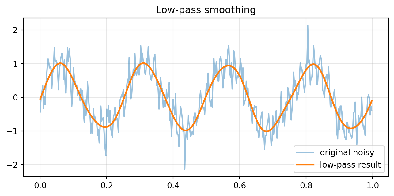
## Worked example 2: low-pass smoothing
A signal has meaningful low-frequency structure plus high-frequency noise. A low-pass filter keeps coefficients with $|f| \leq f_c$ and removes the rest.
```{python}
n = 400
t = np.linspace(0, 1, n, endpoint=False)
rng = np.random.default_rng(8)
x = np.sin(2*np.pi*4*t) + 0.35*np.sin(2*np.pi*50*t) + 0.25*rng.normal(size=n)
X = np.fft.fft(x)
freq = np.fft.fftfreq(n, d=1/n)
cutoff = 10
smoothed = np.fft.ifft(X*(np.abs(freq)<=cutoff)).real

plt.figure(figsize=(8, 3.5))
plt.plot(t, x, alpha=0.45, label='original noisy')
plt.plot(t, smoothed, linewidth=2, label='low-pass result')
plt.legend()
plt.title('Low-pass smoothing')
plt.grid(True, alpha=0.3)
plt.show()
```
## Practice problems
### Problem 1
Let
$$
x = \begin{bmatrix}1\\0\\-1\\0\end{bmatrix}.
$$
Compare this vector with the sampled cosine wave
$$
c = \begin{bmatrix}1\\0\\-1\\0\end{bmatrix}.
$$
Compute $x \cdot c$ and interpret the result.
::: {.callout-tip collapse="true"}
## Solution
$$
x \cdot c = 1^2 + 0^2 + (-1)^2 + 0^2 = 2.
$$
The signal points strongly in the same direction as this wave pattern. In fact, here $x=c$.
:::
### Problem 2
Why is Fourier analysis a change of basis?
::: {.callout-tip collapse="true"}
## Solution
The original coordinates of a signal are time samples. Fourier coordinates describe the same signal using wave coefficients. Since the signal is represented in a different coordinate system, Fourier analysis is a change of basis.
:::
### Problem 3
What is the difference between a low-pass filter and a high-pass filter?
::: {.callout-tip collapse="true"}
## Solution
A low-pass filter keeps low frequencies and removes high frequencies. It usually smooths a signal. A high-pass filter keeps high frequencies and removes low frequencies. It often emphasizes edges, sudden changes, or noise.
:::
### Problem 4
Suppose a signal is very smooth. Would you expect its Fourier coefficients to be mostly low-frequency or high-frequency? Explain.
::: {.callout-tip collapse="true"}
## Solution
A smooth signal changes slowly, so most of its energy is usually in low-frequency coefficients. High-frequency coefficients represent rapid oscillations or sharp changes.
:::
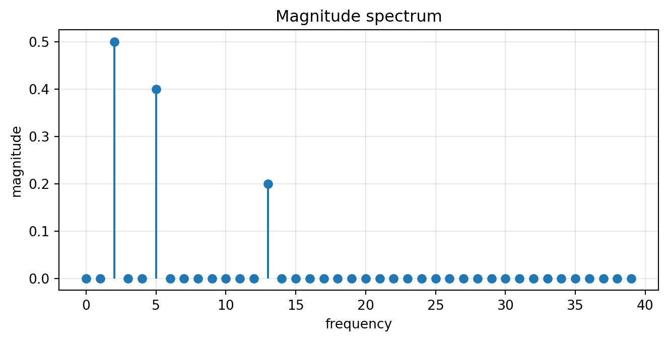
### Problem 5
Use Python to build a signal with frequencies $2$, $5$, and $13$. Compute its FFT and plot the magnitude spectrum.
::: {.callout-tip collapse="true"}
## Solution
```{python}
n = 512
t = np.linspace(0, 1, n, endpoint=False)
x = 1.0*np.cos(2*np.pi*2*t) + 0.8*np.sin(2*np.pi*5*t) + 0.4*np.cos(2*np.pi*13*t)
X = np.fft.fft(x)
freq = np.fft.fftfreq(n, d=1/n)
positive = freq >= 0
plt.figure(figsize=(8, 3.5))
plt.stem(freq[positive][:40], np.abs(X[positive][:40])/n, basefmt=' ')
plt.xlabel('frequency')
plt.ylabel('magnitude')
plt.title('Magnitude spectrum')
plt.grid(True, alpha=0.3)
plt.show()
```
:::
## Challenge questions
1. Why do sharp jumps require many Fourier coefficients to represent accurately?
2. How is Fourier compression similar to projection onto a lower-dimensional subspace?
3. Why might Fourier features help a machine-learning model learn a complicated function?
4. Compare Fourier denoising with PCA denoising. What is fixed? What is learned from data?
5. In image processing, what kinds of visual features correspond to high spatial frequencies?
## AI companion activities
Use an AI assistant as a mathematical conversation partner.
1. Ask it to explain Fourier analysis in three metaphors: music, language, and coordinates.
2. Ask it to generate five signals and predict which frequencies will appear in the FFT.
3. Ask it to compare Fourier, PCA, and SVD using the same example dataset.
4. Ask it to write Python code for a low-pass filter, then inspect every line.
5. Ask it where Fourier analysis appears in speech recognition, MRI, and image compression.
## Chapter summary
Fourier analysis is one of the most important examples of linear algebra in action.
A finite signal is a vector. Wave patterns form a coordinate language. Fourier coefficients measure how much the signal points in each wave direction. The DFT is a matrix transformation, and the FFT is a fast way to compute it. Once a signal is written in frequency coordinates, we can identify hidden frequencies, smooth noise, compress information, and analyze images.
The deepest lesson is this:
::: {.callout-important}
## Final message
Fourier analysis does not merely transform a signal.
It changes the language so that hidden patterns become visible.
:::