---
title: "Chapter 10: Angles and Similarity"
subtitle: "Dot products, cosine similarity, correlation, and the geometry of agreement"
format:
html:
toc: true
toc-depth: 3
number-sections: true
code-fold: true
code-tools: true
jupyter: python3
---
## The story so far
In the last chapter, we learned to measure the **length** of a vector and the **distance** between two points.
Distance answers questions such as:
- How far apart are two data points?
- How large is an error vector?
- Which neighbor is closest?
- How much did a signal change?
But distance is not always the right question.
Suppose two students spend very different amounts of total time studying, but they divide their time across subjects in almost the same proportions. Suppose two documents have very different lengths, but they use words in a similar pattern. Suppose two customers buy very different quantities, but their taste profiles point in the same direction.
In those situations, we do not only care about **how far apart** two vectors are. We care about whether they **point in similar directions**.
That is the central theme of this chapter:
> **Distance compares locations. Angle compares direction. Similarity often lives in the angle.**
Linear algebra gives us a remarkably simple tool for measuring angle: the **dot product**.
## Opening story: two people with similar taste
Suppose Alice rates five movies by
$$
a =
\begin{bmatrix}
5 \\
5 \\
4 \\
1 \\
1
\end{bmatrix},
$$
and Bob rates the same five movies by
$$
b =
\begin{bmatrix}
10 \\
10 \\
8 \\
2 \\
2
\end{bmatrix}.
$$
The two vectors are not equal. Bob uses larger numbers. But Bob's pattern is exactly Alice's pattern:
$$
b = 2a.
$$
The two vectors point in the same direction. They have different lengths, but the same taste profile.
Now suppose Carol rates the movies by
$$
c =
\begin{bmatrix}
1 \\
1 \\
2 \\
5 \\
5
\end{bmatrix}.
$$
Carol's vector points in a different direction. Alice and Bob like the first movies more. Carol likes the last movies more.
A distance calculation sees both size and direction. An angle calculation focuses on direction.
In recommendation systems, text search, clustering, and machine learning, this distinction is essential.
## Learning goals
By the end of this chapter, you should be able to:
1. Compute and interpret the dot product of two vectors.
2. Explain how the dot product detects alignment.
3. Use the formula relating dot product, length, and angle.
4. Compute cosine similarity and interpret its values.
5. Distinguish distance-based comparison from angle-based comparison.
6. Explain orthogonality as zero dot product.
7. Use centering to connect cosine similarity with correlation.
8. Apply similarity ideas to ratings, text vectors, images, and high-dimensional data.
## The dot product: multiplying matching components
Let
$$
u =
\begin{bmatrix}
u_1 \\
u_2 \\
\vdots \\
u_n
\end{bmatrix},
\qquad
v =
\begin{bmatrix}
v_1 \\
v_2 \\
\vdots \\
v_n
\end{bmatrix}.
$$
The **dot product** of $u$ and $v$ is
$$
u \cdot v = u_1v_1 + u_2v_2 + \cdots + u_nv_n.
$$
Equivalently,
$$
u \cdot v = \sum_{i=1}^n u_i v_i.
$$
The dot product multiplies corresponding entries and then adds the results.
::: {.callout-note}
## Interpretation
The dot product measures **coordinated contribution**.
If large positive entries of $u$ occur in the same places as large positive entries of $v$, the dot product becomes large and positive.
If positive entries of one vector align with negative entries of the other, the dot product becomes negative.
If the positive and negative contributions cancel, the dot product may be near zero.
:::
### Example 1: same direction
Let
$$
u = \begin{bmatrix}2 \\ 1\end{bmatrix},
\qquad
v = \begin{bmatrix}6 \\ 3\end{bmatrix}.
$$
Then
$$
u \cdot v = 2(6) + 1(3) = 15.
$$
The dot product is positive and large because the vectors point in the same direction. In fact, $v = 3u$.
### Example 2: opposite direction
Let
$$
u = \begin{bmatrix}2 \\ 1\end{bmatrix},
\qquad
w = \begin{bmatrix}-6 \\ -3\end{bmatrix}.
$$
Then
$$
u \cdot w = 2(-6) + 1(-3) = -15.
$$
The dot product is negative because the vectors point in opposite directions.
### Example 3: perpendicular directions
Let
$$
u = \begin{bmatrix}2 \\ 1\end{bmatrix},
\qquad
z = \begin{bmatrix}-1 \\ 2\end{bmatrix}.
$$
Then
$$
u \cdot z = 2(-1) + 1(2) = 0.
$$
The vectors are perpendicular. Their directions do not reinforce each other.
## Dot product and length
The dot product of a vector with itself gives the squared length:
$$
u \cdot u = u_1^2 + u_2^2 + \cdots + u_n^2 = \|u\|^2.
$$
Therefore,
$$
\|u\| = \sqrt{u \cdot u}.
$$
This is one of the most important bridges in linear algebra:
> The dot product creates the geometry of length, distance, angle, and projection.
### Example
If
$$
u = \begin{bmatrix}3 \\ 4\end{bmatrix},
$$
then
$$
u \cdot u = 3^2 + 4^2 = 25,
$$
so
$$
\|u\| = 5.
$$
## The angle formula
For two nonzero vectors $u$ and $v$, the dot product satisfies
$$
u \cdot v = \|u\|\,\|v\|\cos(\theta),
$$
where $\theta$ is the angle between the vectors.
Solving for $\cos(\theta)$ gives
$$
\cos(\theta) = \frac{u \cdot v}{\|u\|\,\|v\|}.
$$
This formula is the foundation of cosine similarity.
::: {.callout-important}
## What the formula says
The dot product combines three things:
1. the length of $u$,
2. the length of $v$,
3. the cosine of the angle between them.
If we divide by the lengths, we remove size and keep only direction.
:::
## Cosine similarity
The **cosine similarity** between two nonzero vectors $u$ and $v$ is
$$
\operatorname{cosine\_similarity}(u,v)
=
\frac{u \cdot v}{\|u\|\,\|v\|}.
$$
It always lies between $-1$ and $1$.
| Value | Meaning |
|---:|---|
| $1$ | same direction |
| close to $1$ | very similar direction |
| $0$ | perpendicular / unrelated by angle |
| close to $-1$ | nearly opposite direction |
| $-1$ | exactly opposite direction |
In many data applications, especially when entries are nonnegative, cosine similarity usually lies between $0$ and $1$.
### Example: ratings with different scale
Recall
$$
a =
\begin{bmatrix}
5 \\
5 \\
4 \\
1 \\
1
\end{bmatrix},
\qquad
b =
\begin{bmatrix}
10 \\
10 \\
8 \\
2 \\
2
\end{bmatrix}.
$$
Since $b = 2a$, they point in exactly the same direction. Therefore,
$$
\operatorname{cosine\_similarity}(a,b)=1.
$$
Even though Bob's ratings are twice as large, the preference pattern is identical.
### Example: different preference pattern
Let
$$
c =
\begin{bmatrix}
1 \\
1 \\
2 \\
5 \\
5
\end{bmatrix}.
$$
The cosine similarity between $a$ and $c$ is smaller because their large entries occur in different places.
```{python}
import numpy as np

a = np.array([5, 5, 4, 1, 1], dtype=float)
b = np.array([10, 10, 8, 2, 2], dtype=float)
c = np.array([1, 1, 2, 5, 5], dtype=float)

def cosine_similarity(u, v):
    return np.dot(u, v) / (np.linalg.norm(u) * np.linalg.norm(v))

print("cos(a,b) =", cosine_similarity(a,b))
print("cos(a,c) =", cosine_similarity(a,c))
```
## Distance similarity versus angle similarity
Distance and angle answer different questions.
Distance asks:
> How close are the points?
Cosine similarity asks:
> How similar are the directions or patterns?
### Example: short document versus long document
Suppose document $d_1$ has word-count vector
$$
d_1 = \begin{bmatrix}2 \\ 1 \\ 0\end{bmatrix},
$$
and document $d_2$ has
$$
d_2 = \begin{bmatrix}20 \\ 10 \\ 0\end{bmatrix}.
$$
The Euclidean distance is large:
$$
\|d_2-d_1\| = \sqrt{18^2 + 9^2}.
$$
But $d_2 = 10d_1$, so the cosine similarity is $1$.
The two documents have the same word pattern, but different length.
### When should we use distance?
Use distance when magnitude matters:
- physical location,
- measurement error,
- image pixel difference,
- prediction residuals,
- clustering points by absolute position.
### When should we use cosine similarity?
Use cosine similarity when pattern matters more than magnitude:
- document similarity,
- recommendation systems,
- embeddings,
- search ranking,
- comparing normalized feature profiles,
- comparing directions in high-dimensional data.
## Orthogonality: zero similarity by angle
Two nonzero vectors are **orthogonal** if their dot product is zero:
$$
u \cdot v = 0.
$$
Geometrically, this means the angle between them is $90^\circ$.
Since $\cos(90^\circ)=0$, the angle formula gives
$$
u \cdot v = \|u\|\,\|v\|\cos(90^\circ)=0.
$$
Orthogonality means that one direction contributes no component along the other.
::: {.callout-note}
## Orthogonality is stronger than "different"
Two vectors can be different without being orthogonal. Orthogonality means their directions are completely independent in the dot-product sense.
:::
### Example
The vectors
$$
u = \begin{bmatrix}3 \\ 4\end{bmatrix},
\qquad
v = \begin{bmatrix}4 \\ -3\end{bmatrix}
$$
are orthogonal because
$$
u \cdot v = 3(4)+4(-3)=0.
$$
## Projection preview: shadow along a direction
Angles naturally lead to projection.
Suppose $u$ is a vector and $q$ is a unit vector, meaning $\|q\|=1$. The dot product
$$
u \cdot q
$$
measures how much of $u$ lies in the direction of $q$.
The vector
$$
(u \cdot q)q
$$
is the shadow of $u$ onto the direction $q$.
We will study projection deeply in Chapter 11. For now, the important idea is:
> The dot product measures how much one vector points along another vector.
## Centering and correlation
Cosine similarity compares vectors from the origin. But sometimes the origin is not meaningful.
For example, suppose two students have test-score vectors. One student may have higher scores overall, but we may want to compare whether their strengths and weaknesses across topics have similar patterns.
To focus on pattern around each person's average, we first **center** the vectors.
For a vector $x$, define its mean
$$
\bar{x} = \frac{1}{n}\sum_{i=1}^n x_i.
$$
The centered vector is
$$
x - \bar{x}\mathbf{1},
$$
where
$$
\mathbf{1} = \begin{bmatrix}1 \\ 1 \\ \vdots \\ 1\end{bmatrix}.
$$
The correlation between $x$ and $y$ is the cosine similarity of the centered vectors:
$$
\operatorname{corr}(x,y)
=
\frac{(x-\bar{x}\mathbf{1})\cdot(y-\bar{y}\mathbf{1})}
{\|x-\bar{x}\mathbf{1}\|\,\|y-\bar{y}\mathbf{1}\|}.
$$
::: {.callout-important}
## Correlation is centered cosine similarity
Cosine similarity compares directions from the origin.
Correlation compares directions after subtracting each vector's average.
:::
### Example: same pattern with different baseline
Let
$$
x = \begin{bmatrix}70 \\ 80 \\ 90\end{bmatrix},
\qquad
y = \begin{bmatrix}170 \\ 180 \\ 190\end{bmatrix}.
$$
The raw vectors are not the same. But after centering,
$$
x - \bar{x}\mathbf{1} = \begin{bmatrix}-10 \\ 0 \\ 10\end{bmatrix},
$$
and
$$
y - \bar{y}\mathbf{1} = \begin{bmatrix}-10 \\ 0 \\ 10\end{bmatrix}.
$$
So their correlation is $1$.
## Similarity in text data
In text analysis, a document can be represented by a word-count vector.
Suppose we use the vocabulary
$$
[\text{linear},\ \text{matrix},\ \text{recipe},\ \text{movie},\ \text{music}].
$$
A math document might be
$$
d_1 = \begin{bmatrix}5 \\ 4 \\ 2 \\ 0 \\ 0\end{bmatrix},
$$
while another math document might be
$$
d_2 = \begin{bmatrix}10 \\ 9 \\ 3 \\ 0 \\ 0\end{bmatrix}.
$$
A movie-review document might be
$$
d_3 = \begin{bmatrix}0 \\ 0 \\ 0 \\ 6 \\ 4\end{bmatrix}.
$$
Cosine similarity detects that $d_1$ and $d_2$ point in similar directions, while $d_1$ and $d_3$ are nearly orthogonal.
```{python}
vocab = ["linear", "matrix", "recipe", "movie", "music"]
d1 = np.array([5, 4, 2, 0, 0], dtype=float)
d2 = np.array([10, 9, 3, 0, 0], dtype=float)
d3 = np.array([0, 0, 0, 6, 4], dtype=float)

print("cos(d1,d2) =", cosine_similarity(d1,d2))
print("cos(d1,d3) =", cosine_similarity(d1,d3))
```
This is the beginning of the vector-space model for search engines and modern embedding methods.
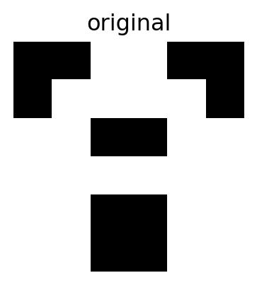
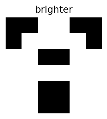
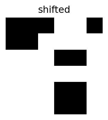
## Similarity in images
An image can be flattened into a vector. Two images are similar if their pixel vectors point in similar directions or are close in distance.
However, cosine similarity and distance can behave differently.
- Distance is sensitive to brightness changes.
- Cosine similarity is less sensitive to multiplying all pixels by the same positive constant.
```{python}
import matplotlib.pyplot as plt

img = np.array([
    [0,0,1,1,0,0],
    [0,1,1,1,1,0],
    [1,1,0,0,1,1],
    [1,1,1,1,1,1],
    [1,1,0,0,1,1],
    [1,1,0,0,1,1]
], dtype=float)

bright = 2 * img
shifted = np.roll(img, 1, axis=1)

for title, image in [("original", img), ("brighter", bright), ("shifted", shifted)]:
    plt.figure(figsize=(2.2,2.2))
    plt.imshow(image, cmap="gray")
    plt.title(title)
    plt.axis("off")
    plt.show()

print("cos(original, brighter) =", cosine_similarity(img.ravel(), bright.ravel()))
print("cos(original, shifted) =", cosine_similarity(img.ravel(), shifted.ravel()))
print("distance(original, brighter) =", np.linalg.norm(img.ravel() - bright.ravel()))
print("distance(original, shifted) =", np.linalg.norm(img.ravel() - shifted.ravel()))
```
This example shows that similarity depends on the question. If brightness should not matter, cosine similarity may be useful. If pixel-by-pixel difference matters, distance may be better.
## High-dimensional angles
High-dimensional geometry can be surprising.
If we choose two random high-dimensional vectors, they are often nearly orthogonal. That means their cosine similarity is often close to $0$.
This is not because the vectors are simple. It is because in high dimensions, there are many independent directions.
```{python}
import numpy as np
import matplotlib.pyplot as plt

rng = np.random.default_rng(0)

for d in [2, 10, 100, 1000]:
    X = rng.normal(size=(3000, d))
    Y = rng.normal(size=(3000, d))
    dots = np.sum(X * Y, axis=1)
    norms = np.linalg.norm(X, axis=1) * np.linalg.norm(Y, axis=1)
    cosines = dots / norms
    print(f"dimension {d:4d}: mean={cosines.mean(): .4f}, std={cosines.std(): .4f}")
```
As the dimension increases, random directions concentrate near perpendicularity.
::: {.callout-warning}
## High-dimensional warning
In high dimensions, small differences in cosine similarity may be meaningful. A cosine similarity of $0.2$ may indicate much stronger alignment than it sounds like, especially when random vectors tend to have cosine similarity near $0$.
:::
## The dot product as a score
Many machine-learning models use dot products as scores.
If $x$ is a feature vector and $w$ is a weight vector, then
$$
s = w \cdot x
$$
is a score.
The score is large when $x$ points strongly in the direction that $w$ values.
For example, if
$$
w =
\begin{bmatrix}
2 \\
-1 \\
3
\end{bmatrix},
$$
then the score
$$
w \cdot x = 2x_1 - x_2 + 3x_3
$$
rewards large $x_1$ and $x_3$, but penalizes large $x_2$.
This is the seed of linear classifiers, regression models, neural network layers, attention mechanisms, and recommendation models.
## Worked example: comparing study patterns
Three students record weekly study hours in four subjects:
$$
A = \begin{bmatrix}8 \\ 6 \\ 2 \\ 2\end{bmatrix},
\qquad
B = \begin{bmatrix}16 \\ 12 \\ 4 \\ 4\end{bmatrix},
\qquad
C = \begin{bmatrix}2 \\ 2 \\ 8 \\ 6\end{bmatrix}.
$$
Student $B$ studies twice as much as student $A$ in every subject, so their cosine similarity is $1$.
Student $C$ spends more time on the last two subjects, so the similarity with $A$ is smaller.
```{python}
A = np.array([8, 6, 2, 2], dtype=float)
B = np.array([16, 12, 4, 4], dtype=float)
C = np.array([2, 2, 8, 6], dtype=float)

print("cos(A,B) =", cosine_similarity(A,B))
print("cos(A,C) =", cosine_similarity(A,C))
print("dist(A,B) =", np.linalg.norm(A-B))
print("dist(A,C) =", np.linalg.norm(A-C))
```
Notice that $A$ may be closer in distance to $C$ than to $B$, while more similar in direction to $B$. This is the core distinction.
## Practice problems
### Problem 1
Compute $u \cdot v$ for
$$
u = \begin{bmatrix}1 \\ 2 \\ 3\end{bmatrix},
\qquad
v = \begin{bmatrix}4 \\ -1 \\ 2\end{bmatrix}.
$$
::: {.callout-tip collapse="true"}
## Solution
$$
u \cdot v = 1(4)+2(-1)+3(2)=4-2+6=8.$$
:::
### Problem 2
Find the cosine similarity between
$$
u = \begin{bmatrix}1 \\ 0\end{bmatrix},
\qquad
v = \begin{bmatrix}1 \\ 1\end{bmatrix}.
$$
::: {.callout-tip collapse="true"}
## Solution
We have
$$
u \cdot v = 1,$$
$$
\|u\|=1,
\qquad
\|v\|=\sqrt{2}.
$$
So
$$
\operatorname{cosine\_similarity}(u,v)=\frac{1}{\sqrt{2}}.
$$
The angle is $45^\circ$.
:::
### Problem 3
Find a nonzero vector orthogonal to
$$
u = \begin{bmatrix}5 \\ 2\end{bmatrix}.
$$
::: {.callout-tip collapse="true"}
## Solution
One answer is
$$
v = \begin{bmatrix}2 \\ -5\end{bmatrix}.
$$
Then
$$
u \cdot v = 5(2)+2(-5)=10-10=0.$$
:::
### Problem 4
Let
$$
x = \begin{bmatrix}1 \\ 2 \\ 3\end{bmatrix},
\qquad
y = \begin{bmatrix}11 \\ 12 \\ 13\end{bmatrix}.
$$
Compute the centered vectors and explain why the correlation is $1$.
::: {.callout-tip collapse="true"}
## Solution
The means are $\bar{x}=2$ and $\bar{y}=12$.
The centered vectors are
$$
x-\bar{x}\mathbf{1}
=
\begin{bmatrix}-1 \\ 0 \\ 1\end{bmatrix},
\qquad
y-\bar{y}\mathbf{1}
=
\begin{bmatrix}-1 \\ 0 \\ 1\end{bmatrix}.
$$
They are the same centered vector, so their cosine similarity is $1$. Therefore their correlation is $1$.
:::
### Problem 5
Give an example of two nonzero vectors whose cosine similarity is $1$ but whose Euclidean distance is not $0$.
::: {.callout-tip collapse="true"}
## Solution
One example is
$$
u = \begin{bmatrix}1 \\ 2\end{bmatrix},
\qquad
v = \begin{bmatrix}2 \\ 4\end{bmatrix}.
$$
They point in the same direction, so cosine similarity is $1$. But
$$
\|u-v\| = \sqrt{1^2+2^2}=\sqrt{5},
$$
so their distance is not $0$.
:::
## Python lab preview
The accompanying notebook for this chapter explores:
- dot products as alignment scores,
- cosine similarity and angle,
- distance versus cosine similarity,
- correlation as centered cosine similarity,
- document similarity,
- image similarity,
- random high-dimensional angles,
- nearest-neighbor search using cosine similarity.
## AI companion activities
Use an AI assistant as a mathematical conversation partner.
1. Ask it to explain the difference between distance and cosine similarity using three examples: ratings, text documents, and images.
2. Ask it to generate two vectors with high cosine similarity but large Euclidean distance.
3. Ask it to generate two vectors with small Euclidean distance but noticeably different cosine similarity.
4. Ask it to explain why random high-dimensional vectors are often nearly orthogonal.
5. Ask it to design a small recommendation-system example using cosine similarity.
When using AI, always check the computations yourself. The purpose is not to outsource thinking. The purpose is to create more examples, test your understanding, and ask better questions.
## Chapter summary
This chapter introduced the geometry of direction.
- The dot product is $u \cdot v = \sum_i u_i v_i$.
- The length of a vector is determined by $\|u\| = \sqrt{u\cdot u}$.
- The dot product satisfies $u\cdot v = \|u\|\,\|v\|\cos(\theta)$.
- Cosine similarity removes length and compares direction.
- Orthogonal vectors have dot product $0$.
- Correlation is cosine similarity after centering.
- Text, recommendations, image comparison, and machine learning all use similarity ideas.
- In high dimensions, random vectors are often nearly orthogonal.
Distance tells us how far apart two points are. Angle tells us whether they point in the same direction.
Together, distance and angle form the beginning of geometric thinking in data science and applied linear algebra.