---
title: "Chapter 6: Stretching, Rotating, and Shearing"
subtitle: "How matrices reshape the plane"
format:
html:
toc: true
toc-depth: 3
number-sections: true
code-fold: true
code-tools: true
jupyter: python3
---
## Opening story: the invisible machine behind a moving picture
Imagine that a photograph is printed on a perfectly elastic sheet.
You can pull the sheet horizontally. The photograph becomes wider. You can pull it vertically. The photograph becomes taller. You can rotate the sheet. The photograph turns without changing its shape. You can push the top edge sideways while holding the bottom edge fixed. A square becomes a slanted parallelogram. You can flip the sheet across a mirror line. Left and right switch places.
All of these actions feel physical. But each of them can also be described by a small table of numbers:
$$
A=
\begin{bmatrix}
a & b\\
c & d
\end{bmatrix}.
$$
This is the surprising idea of the chapter:
> A $2\times 2$ matrix is not just an array of four numbers. It is a rule for reshaping the entire plane.
In Chapter 5, a matrix was a machine:
$$
x \longmapsto Ax.
$$
Now we watch what that machine does to space itself. We will not only compute $Ax$ for one vector. We will ask what happens to every point, every arrow, every grid line, every square, every circle, and every cloud of data.
The main message is simple:
> To understand a matrix, watch how it moves the standard basis vectors and how it reshapes a grid.
## Learning goals
By the end of this chapter, you should be able to:
1. Interpret a $2\times 2$ matrix as a transformation of the plane.
2. Explain why the columns of a matrix tell where the standard basis vectors go.
3. Recognize stretching, reflection, rotation, and shear from a matrix.
4. Describe how a unit square becomes a parallelogram.
5. Connect determinant to signed area change and orientation.
6. Understand composition of transformations through matrix multiplication.
7. Use Python to visualize transformations of points, grids, images, and data clouds.
8. Explain why geometric transformation is a foundation for computer graphics, image processing, robotics, and machine learning.
## 6.1 The plane as a stage
A point in the plane is represented by a vector
$$
x=
\begin{bmatrix}
x_1\\
x_2
\end{bmatrix}.
$$
A $2\times 2$ matrix
$$
A=
\begin{bmatrix}
a & b\\
c & d
\end{bmatrix}
$$
sends this point to
$$
Ax=
\begin{bmatrix}
a & b\\
c & d
\end{bmatrix}
\begin{bmatrix}
x_1\\
x_2
\end{bmatrix}
=
\begin{bmatrix}
ax_1+bx_2\\
cx_1+dx_2
\end{bmatrix}.
$$
The formula is important, but the geometry is more memorable. The matrix tells each point where to go.
::: {.callout-note}
## Mental picture
Think of the plane as a sheet covered by a grid. A matrix transformation moves every point on the sheet. Straight grid lines remain straight. Parallel grid lines remain parallel. The origin stays fixed.
:::
A transformation with these properties is called a **linear transformation** of the plane.
::: {.callout-important}
## Definition: linear transformation in the plane
A function $T:\mathbb R^2\to\mathbb R^2$ is linear if
$$
T(u+v)=T(u)+T(v)
$$
and
$$
T(cu)=cT(u)
$$
for all vectors $u,v\in\mathbb R^2$ and all scalars $c$.
Every $2\times 2$ matrix defines a linear transformation by $T(x)=Ax$.
:::
Linearity means the transformation respects addition and scaling. If you first combine two arrows and then transform, you get the same result as transforming the arrows first and then combining them.
## 6.2 The most important diagnostic: where do $e_1$ and $e_2$ go?
The standard basis vectors are
$$
e_1=
\begin{bmatrix}1\\0\end{bmatrix},
\qquad
e_2=
\begin{bmatrix}0\\1\end{bmatrix}.
$$
For
$$
A=
\begin{bmatrix}
a & b\\
c & d
\end{bmatrix},
$$
we have
$$
Ae_1=
\begin{bmatrix}a\\c\end{bmatrix},
\qquad
Ae_2=
\begin{bmatrix}b\\d\end{bmatrix}.
$$
So the first column of $A$ is where $e_1$ goes. The second column of $A$ is where $e_2$ goes.
This is the key to the whole chapter.
::: {.callout-tip}
## Column interpretation
The matrix
$$
A=
\begin{bmatrix}
| & |\\
Ae_1 & Ae_2\\
| & |
\end{bmatrix}
$$
stores the images of the two standard basis vectors as its columns.
:::
Why is this enough? Every vector can be written as
$$
x=
\begin{bmatrix}x_1\\x_2\end{bmatrix}=x_1e_1+x_2e_2.
$$
Using linearity,
$$
Ax=A(x_1e_1+x_2e_2)=x_1Ae_1+x_2Ae_2.
$$
So once we know where $e_1$ and $e_2$ go, we know where every vector goes.
## 6.3 A Python toolkit for seeing matrix transformations
The following code creates helper functions. We will use them to transform vectors, grids, squares, circles, and data clouds.
```{python}
import numpy as np
import matplotlib.pyplot as plt

np.set_printoptions(precision=3, suppress=True)

def transform_points(A, points):
    """Transform an array of 2D points by matrix A.
    points has shape (n, 2). The result also has shape (n, 2).
    """
    A = np.asarray(A, dtype=float)
    points = np.asarray(points, dtype=float)
    return points @ A.T


def draw_axes(ax, lim=4):
    ax.axhline(0, linewidth=1)
    ax.axvline(0, linewidth=1)
    ax.set_xlim(-lim, lim)
    ax.set_ylim(-lim, lim)
    ax.set_aspect("equal", adjustable="box")
    ax.grid(True, alpha=0.3)
    ax.set_xlabel("$x_1$")
    ax.set_ylabel("$x_2$")


def plot_basis(A, lim=4, title="Images of the standard basis"):
    A = np.asarray(A, dtype=float)
    e1 = np.array([1, 0])
    e2 = np.array([0, 1])
    Ae1 = A @ e1
    Ae2 = A @ e2

    fig, ax = plt.subplots(figsize=(6, 6))
    draw_axes(ax, lim=lim)
    ax.quiver(0, 0, e1[0], e1[1], angles="xy", scale_units="xy", scale=1, label="$e_1$")
    ax.quiver(0, 0, e2[0], e2[1], angles="xy", scale_units="xy", scale=1, label="$e_2$")
    ax.quiver(0, 0, Ae1[0], Ae1[1], angles="xy", scale_units="xy", scale=1, label="$Ae_1$")
    ax.quiver(0, 0, Ae2[0], Ae2[1], angles="xy", scale_units="xy", scale=1, label="$Ae_2$")
    ax.set_title(title)
    ax.legend(loc="upper left")
    plt.show()


def plot_grid(A, lim=3, n_lines=13, title="Grid transformation"):
    A = np.asarray(A, dtype=float)
    values = np.linspace(-lim, lim, n_lines)
    fig, ax = plt.subplots(figsize=(7, 7))
    draw_axes(ax, lim=lim * 2)

    for v in values:
        horizontal = np.column_stack([np.linspace(-lim, lim, 200), np.full(200, v)])
        vertical = np.column_stack([np.full(200, v), np.linspace(-lim, lim, 200)])
        Th = transform_points(A, horizontal)
        Tv = transform_points(A, vertical)
        ax.plot(Th[:, 0], Th[:, 1], linewidth=0.8, alpha=0.7)
        ax.plot(Tv[:, 0], Tv[:, 1], linewidth=0.8, alpha=0.7)

    ax.set_title(title)
    plt.show()


def plot_shape(A, points, lim=4, title="Shape transformation"):
    A = np.asarray(A, dtype=float)
    points = np.asarray(points, dtype=float)
    Tpoints = transform_points(A, points)

    fig, ax = plt.subplots(figsize=(7, 7))
    draw_axes(ax, lim=lim)
    ax.plot(points[:, 0], points[:, 1], marker="o", label="original")
    ax.plot(Tpoints[:, 0], Tpoints[:, 1], marker="o", label="transformed")
    ax.set_title(title)
    ax.legend()
    plt.show()

square = np.array([
    [0, 0],
    [1, 0],
    [1, 1],
    [0, 1],
    [0, 0]
])
```
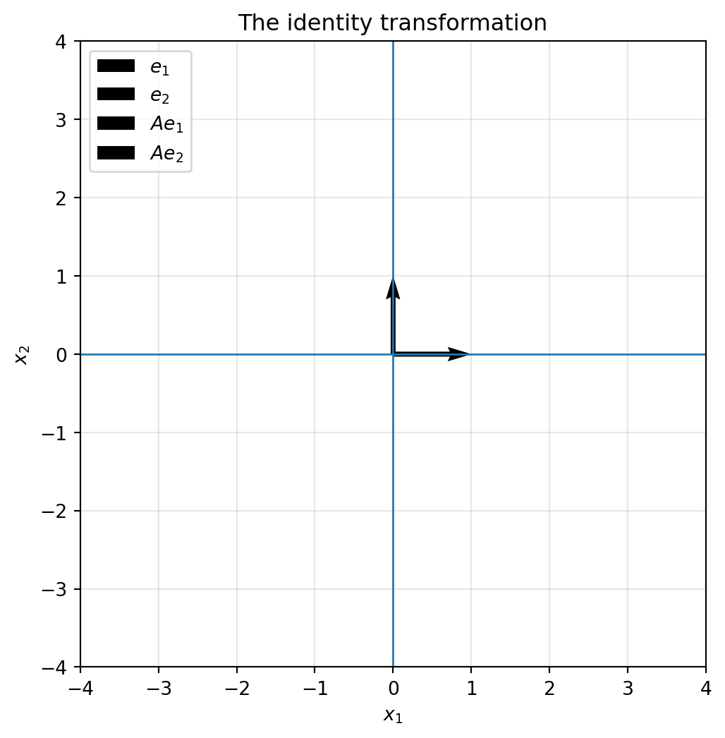
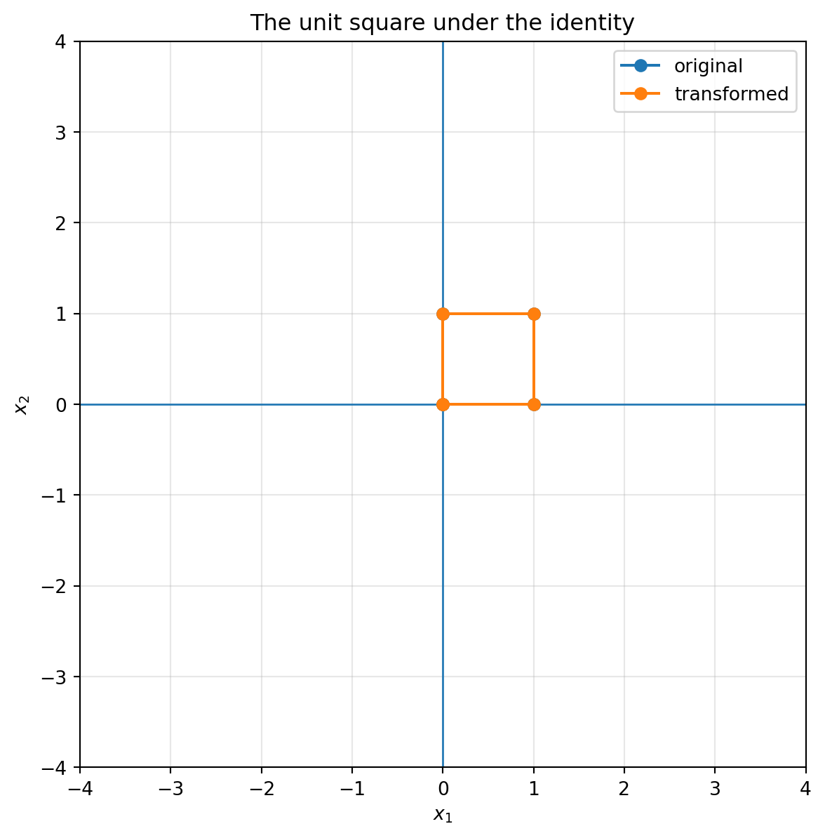
## 6.4 Identity: doing nothing is still a transformation
The identity matrix is
$$
I=
\begin{bmatrix}
1 & 0\\
0 & 1
\end{bmatrix}.
$$
It sends every vector to itself:
$$
Ix=x.
$$
```{python}
I = np.array([[1, 0],
              [0, 1]])

plot_basis(I, title="The identity transformation")
plot_shape(I, square, title="The unit square under the identity")
```
The identity transformation is useful because it gives us a reference point. Every other matrix can be understood as a way of changing the identity grid.
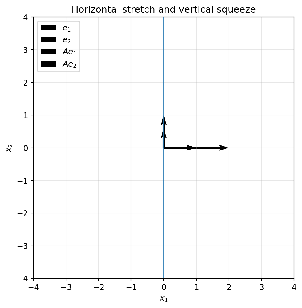
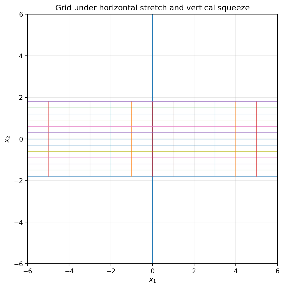
## 6.5 Stretching and squeezing
A diagonal matrix
$$
A=
\begin{bmatrix}
s_x & 0\\
0 & s_y
\end{bmatrix}
$$
scales the horizontal and vertical directions separately:
$$
\begin{bmatrix}
s_x & 0\\
0 & s_y
\end{bmatrix}
\begin{bmatrix}
x_1\\x_2
\end{bmatrix}
=
\begin{bmatrix}
s_xx_1\\s_yx_2
\end{bmatrix}.
$$
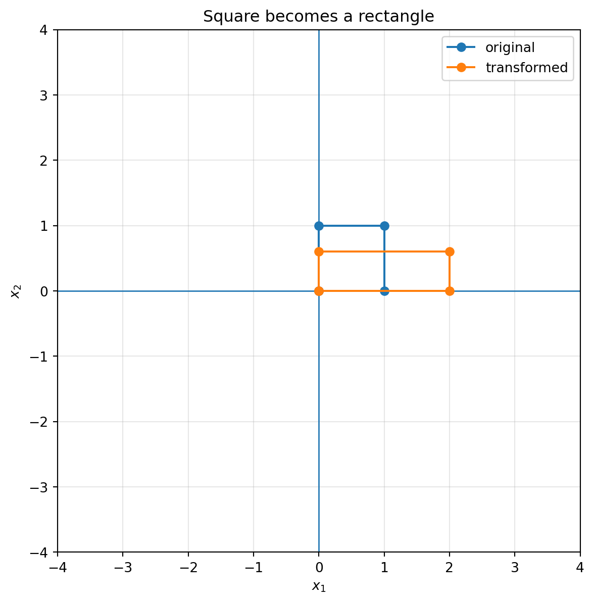
If $s_x>1$, the plane stretches horizontally. If $0<s_x<1$, the plane squeezes horizontally. Negative values also flip direction.
```{python}
A_stretch = np.array([[2.0, 0.0],
                      [0.0, 0.6]])

plot_basis(A_stretch, title="Horizontal stretch and vertical squeeze")
plot_grid(A_stretch, title="Grid under horizontal stretch and vertical squeeze")
plot_shape(A_stretch, square, title="Square becomes a rectangle")
```
::: {.callout-note}
## Interpretation
The matrix
$$
\begin{bmatrix}
2 & 0\\
0 & 0.6
\end{bmatrix}
$$
sends $e_1$ to $(2,0)$ and $e_2$ to $(0,0.6)$. The square becomes a rectangle. Lengths change, but horizontal and vertical directions stay perpendicular.
:::
## 6.6 Reflection: flipping space
A reflection flips the plane across a line.
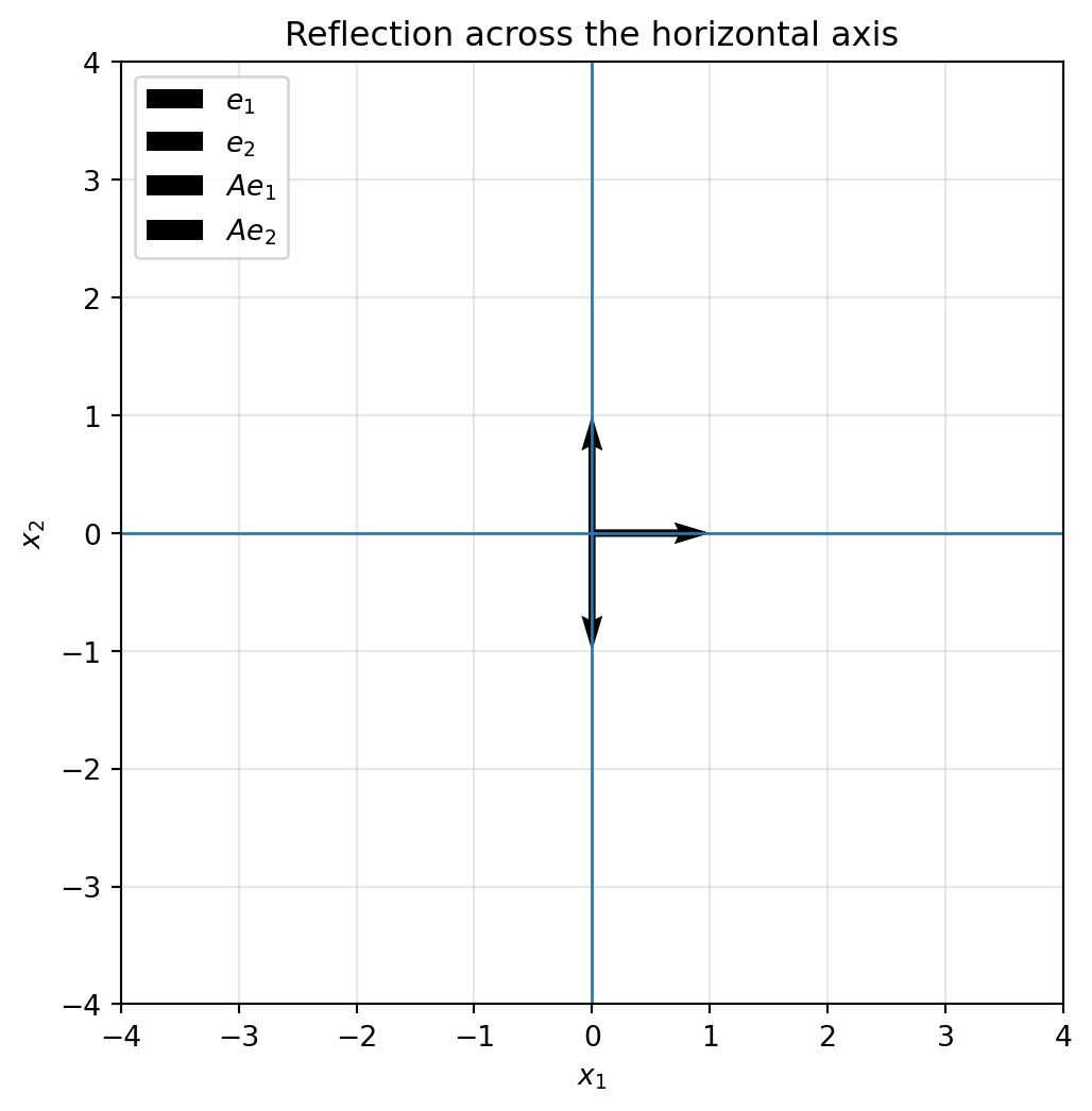
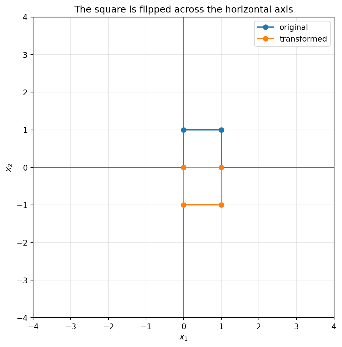
Reflection across the $x_1$-axis is
$$
R_x=
\begin{bmatrix}
1 & 0\\
0 & -1
\end{bmatrix}.
$$
It sends
$$
\begin{bmatrix}x_1\\x_2\end{bmatrix}
\mapsto
\begin{bmatrix}x_1\\-x_2\end{bmatrix}.
$$
Reflection across the $x_2$-axis is
$$
R_y=
\begin{bmatrix}
-1 & 0\\
0 & 1
\end{bmatrix}.
$$
```{python}
R_x = np.array([[1, 0],
                [0, -1]])

plot_basis(R_x, title="Reflection across the horizontal axis")
plot_shape(R_x, square, title="The square is flipped across the horizontal axis")
```
Reflection is one of the first examples where orientation matters. A counterclockwise loop can become clockwise after reflection.
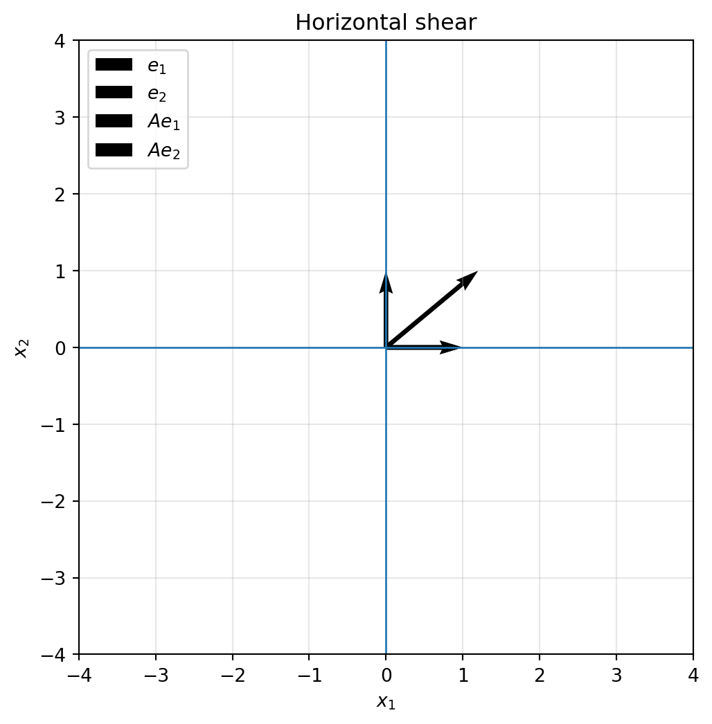
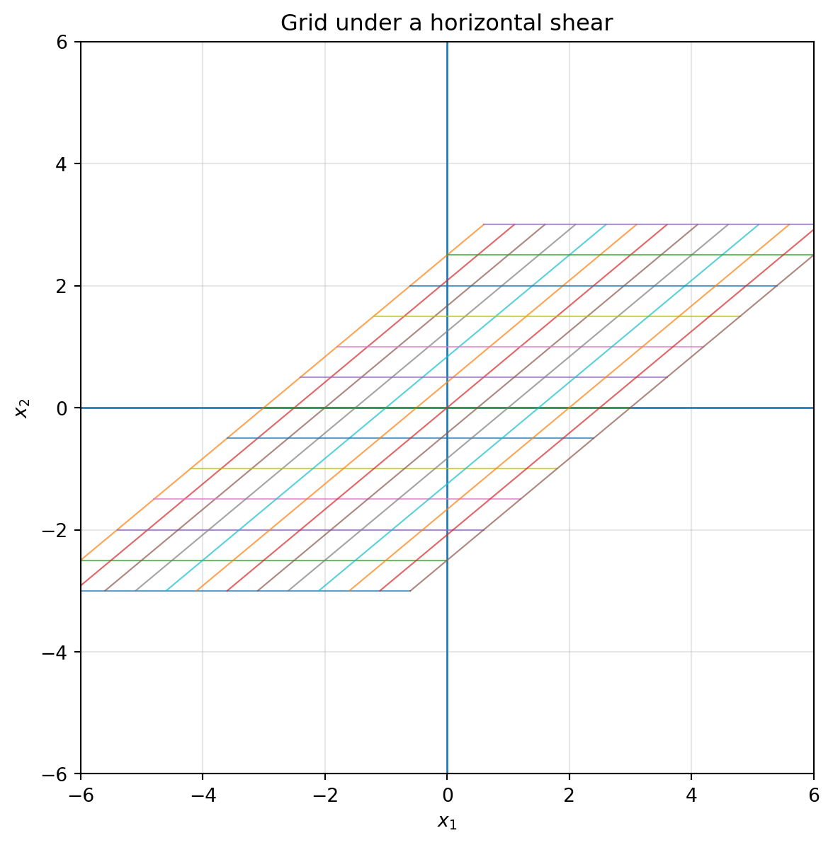
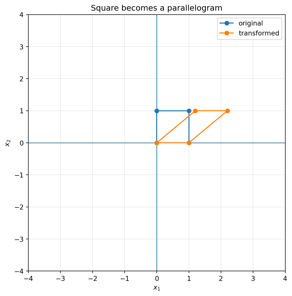
## 6.7 Shear: sliding one direction along another
A shear transformation slants space without necessarily changing area.
A horizontal shear has the form
$$
S_h=
\begin{bmatrix}
1 & k\\
0 & 1
\end{bmatrix}.
$$
It sends
$$
\begin{bmatrix}x_1\\x_2\end{bmatrix}
\mapsto
\begin{bmatrix}x_1+kx_2\\x_2\end{bmatrix}.
$$
The higher a point is, the more it slides horizontally.
```{python}
S_h = np.array([[1.0, 1.2],
                [0.0, 1.0]])

plot_basis(S_h, title="Horizontal shear")
plot_grid(S_h, title="Grid under a horizontal shear")
plot_shape(S_h, square, title="Square becomes a parallelogram")
```
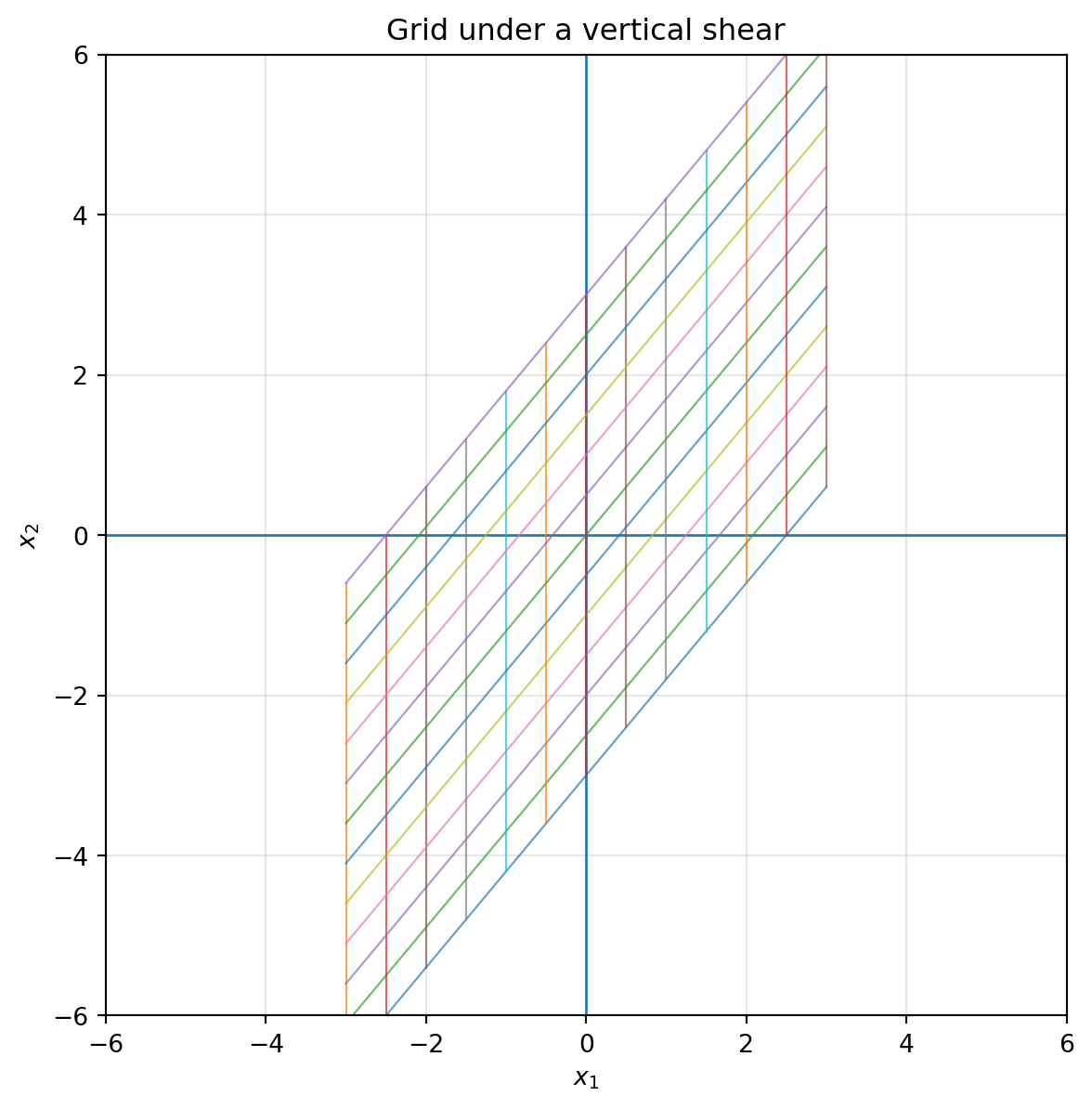
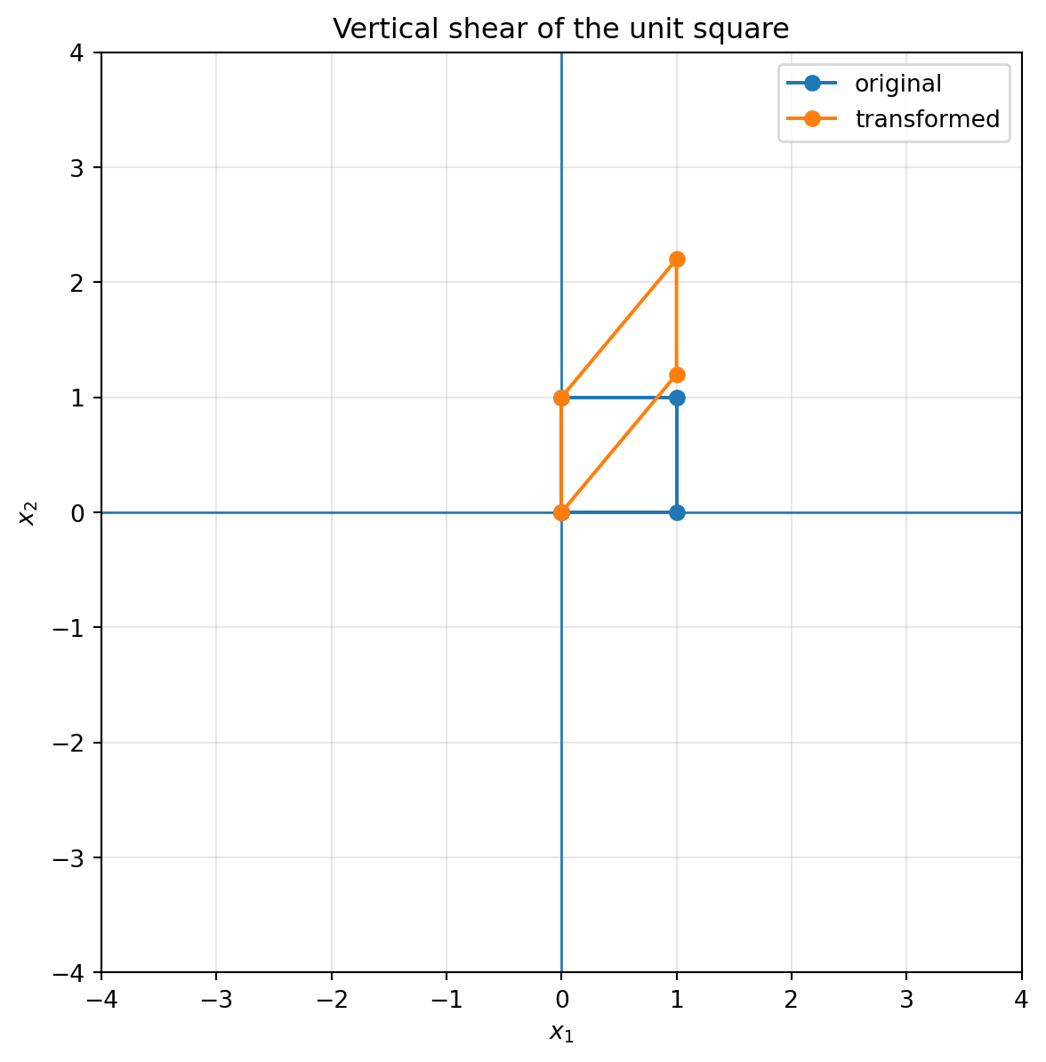
A vertical shear has the form
$$
S_v=
\begin{bmatrix}
1 & 0\\
k & 1
\end{bmatrix}.
$$
It sends
$$
\begin{bmatrix}x_1\\x_2\end{bmatrix}
\mapsto
\begin{bmatrix}x_1\\kx_1+x_2\end{bmatrix}.
$$
The farther right a point is, the more it slides vertically.
```{python}
S_v = np.array([[1.0, 0.0],
                [1.2, 1.0]])

plot_grid(S_v, title="Grid under a vertical shear")
plot_shape(S_v, square, title="Vertical shear of the unit square")
```
::: {.callout-tip}
## How to recognize shear
A shear keeps one basis vector fixed and moves the other by adding some multiple of the fixed direction.
For example,
$$
\begin{bmatrix}
1 & k\\
0 & 1
\end{bmatrix}
$$
keeps $e_1$ fixed and sends $e_2$ to $ke_1+e_2$.
:::
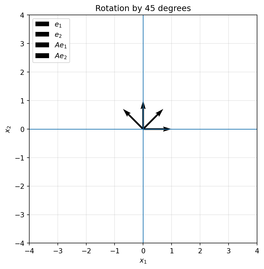
## 6.8 Rotation: turning without stretching
A rotation by angle $\theta$ counterclockwise is represented by
$$
R_\theta=
\begin{bmatrix}
\cos\theta & -\sin\theta\\
\sin\theta & \cos\theta
\end{bmatrix}.
$$
It sends
$$
e_1 \mapsto
\begin{bmatrix}
\cos\theta\\
\sin\theta
\end{bmatrix},
\qquad
e_2 \mapsto
\begin{bmatrix}
-\sin\theta\\
\cos\theta
\end{bmatrix}.
$$
So the two basis vectors rotate together while staying perpendicular and keeping length $1$.
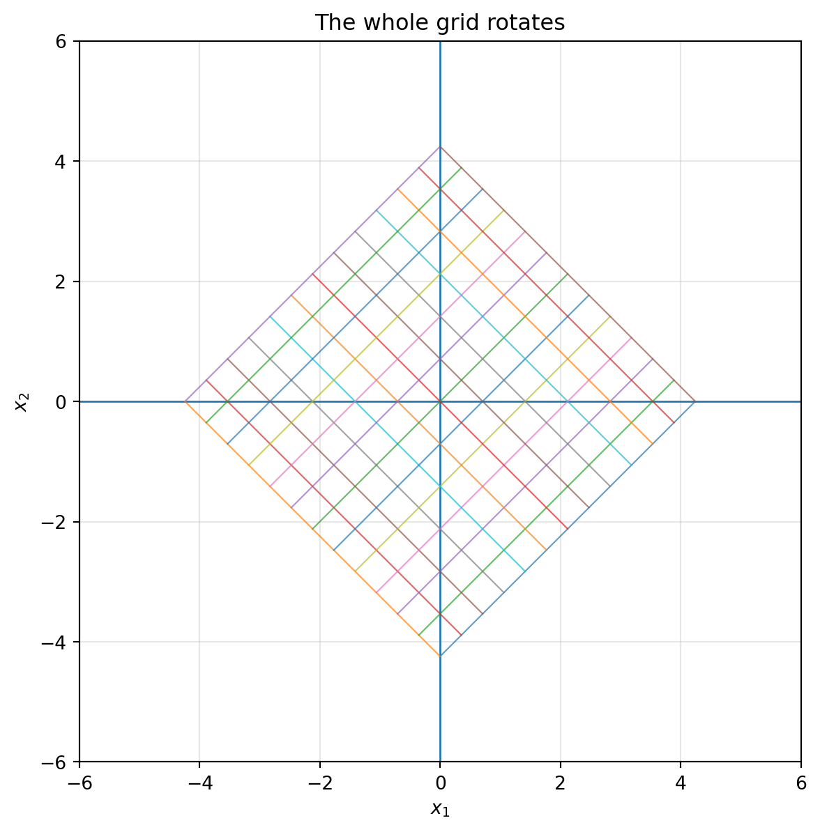
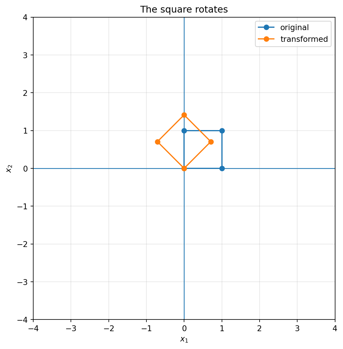
```{python}
theta = np.pi / 4
R = np.array([[np.cos(theta), -np.sin(theta)],
              [np.sin(theta),  np.cos(theta)]])

plot_basis(R, title="Rotation by 45 degrees")
plot_grid(R, title="The whole grid rotates")
plot_shape(R, square, title="The square rotates")
```
::: {.callout-note}
## Rotation preserves geometry
A rotation preserves lengths, angles, distances, and areas. It changes position and direction, but it does not distort shape.
:::
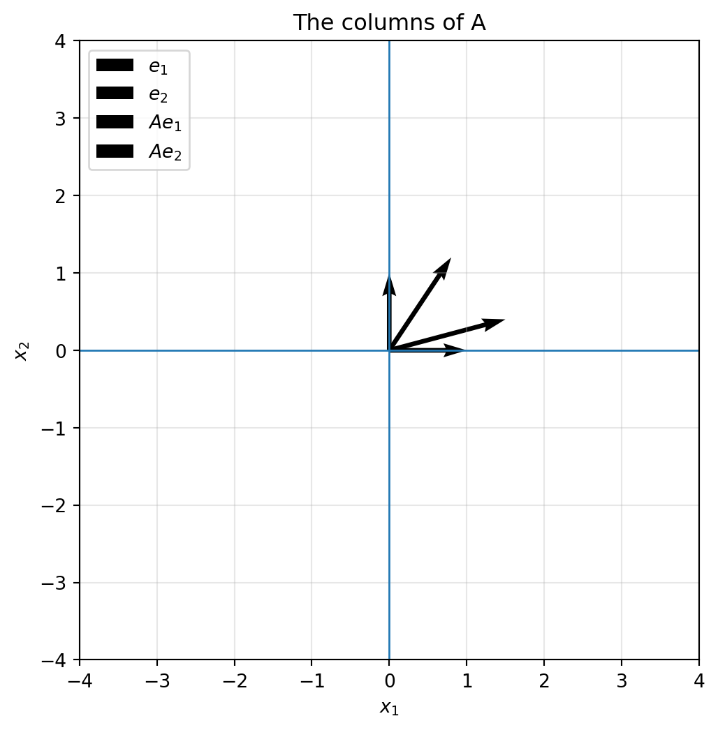
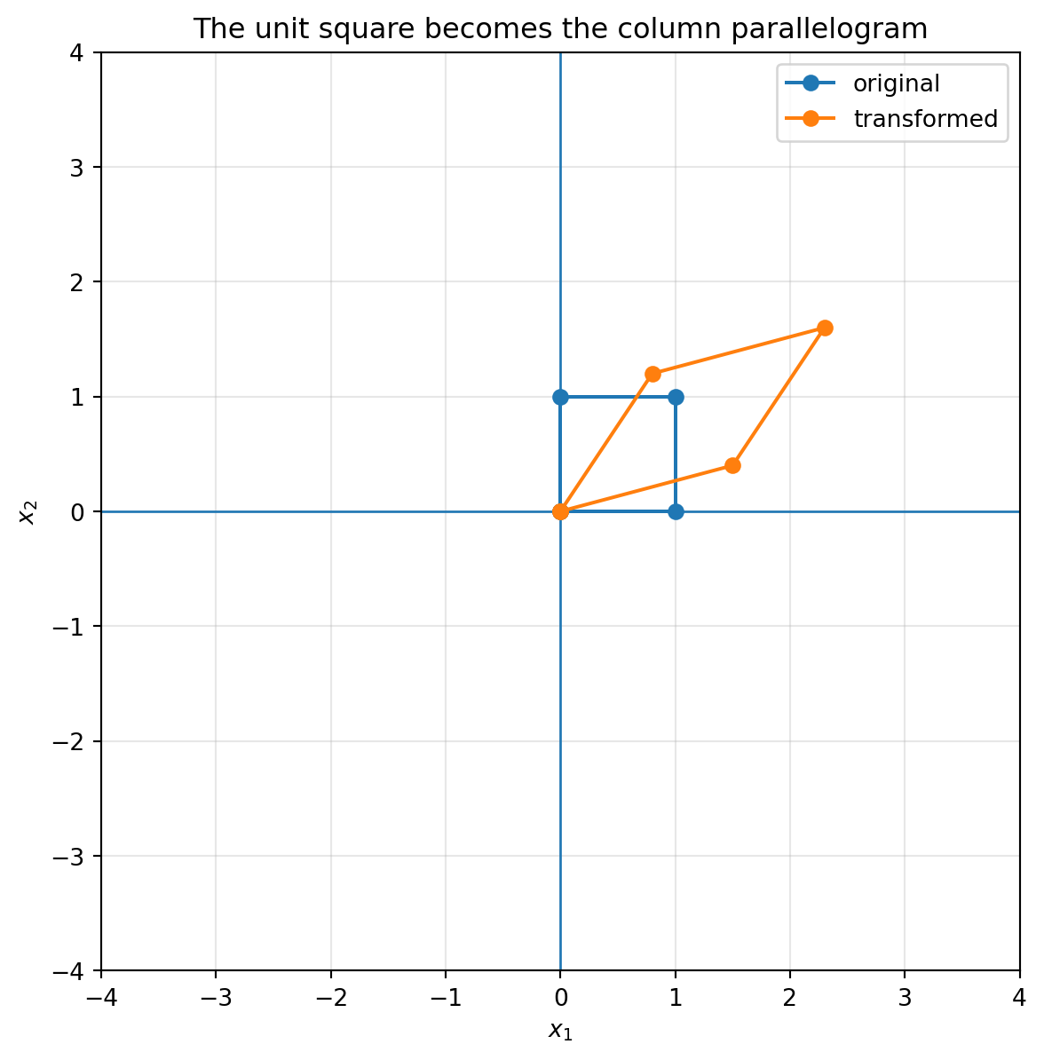
## 6.9 The unit square becomes the column parallelogram
The unit square has corners
$$
0,
\quad e_1,
\quad e_1+e_2,
\quad e_2.
$$
After applying $A$, these corners become
$$
0,
\quad Ae_1,
\quad Ae_1+Ae_2,
\quad Ae_2.
$$
So the unit square becomes the parallelogram spanned by the columns of $A$.
```{python}
A = np.array([[1.5, 0.8],
              [0.4, 1.2]])

plot_basis(A, title="The columns of A")
plot_shape(A, square, title="The unit square becomes the column parallelogram")
```
This picture is one of the most important in all of linear algebra. It connects columns, combinations, geometry, and area.
## 6.10 Determinant: signed area change
For
$$
A=\begin{bmatrix}a & b\\ c & d\end{bmatrix},
$$
the determinant is
$$
\det(A)=ad-bc.
$$
Geometrically, $|\det(A)|$ is the area of the parallelogram formed by the columns of $A$.
More generally:
> Applying $A$ multiplies every area in the plane by $|\det(A)|$.
The sign of $\det(A)$ tells whether orientation is preserved or reversed.
- If $\det(A)>0$, orientation is preserved.
- If $\det(A)<0$, orientation is reversed.
- If $\det(A)=0$, area collapses to zero, so information is lost.
```{python}
matrices = {
    "stretch": np.array([[2, 0], [0, 0.5]]),
    "shear": np.array([[1, 1.5], [0, 1]]),
    "reflection": np.array([[1, 0], [0, -1]]),
    "collapse": np.array([[1, 2], [2, 4]])
}

for name, M in matrices.items():
    print(name, "determinant =", np.linalg.det(M))
```
::: {.callout-important}
## Determinant as geometric information
The determinant is not just a formula. It tells how the matrix changes area and orientation.
$$
|\det(A)|=\text{area-scaling factor}.
$$
When $\det(A)=0$, the transformed unit square has zero area. The plane has been collapsed onto a line or a point.
:::
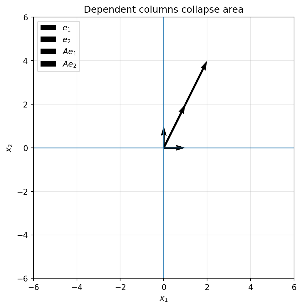
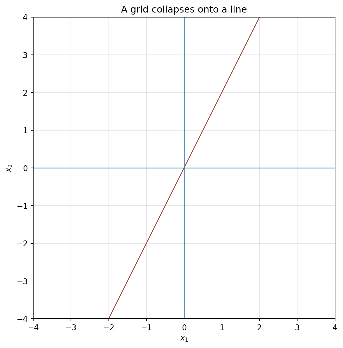
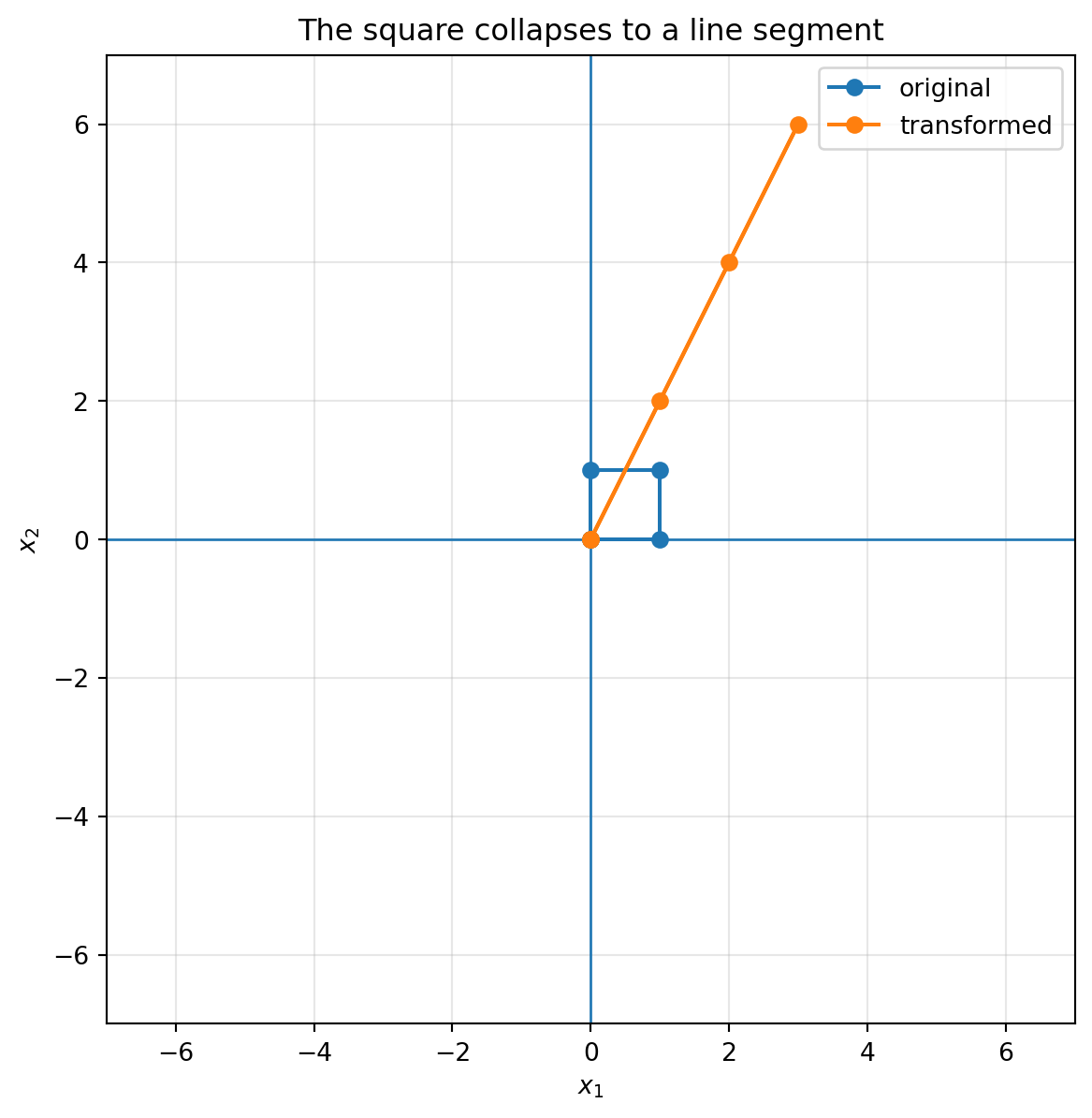
## 6.11 When a matrix collapses space
Consider
$$
C=
\begin{bmatrix}
1 & 2\\
2 & 4
\end{bmatrix}.
$$
The second column is twice the first column. Therefore the two column directions do not span a full parallelogram. They lie on the same line.
```{python}
C = np.array([[1, 2],
              [2, 4]])

plot_basis(C, lim=6, title="Dependent columns collapse area")
plot_grid(C, lim=2, title="A grid collapses onto a line")
plot_shape(C, square, lim=7, title="The square collapses to a line segment")
```
This is the geometric meaning of a zero determinant.
The matrix still transforms vectors, but it loses information. Many different input points land on the same output line.
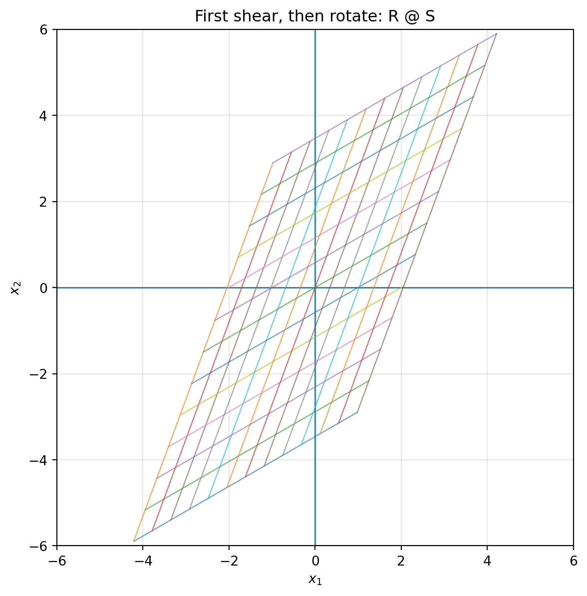
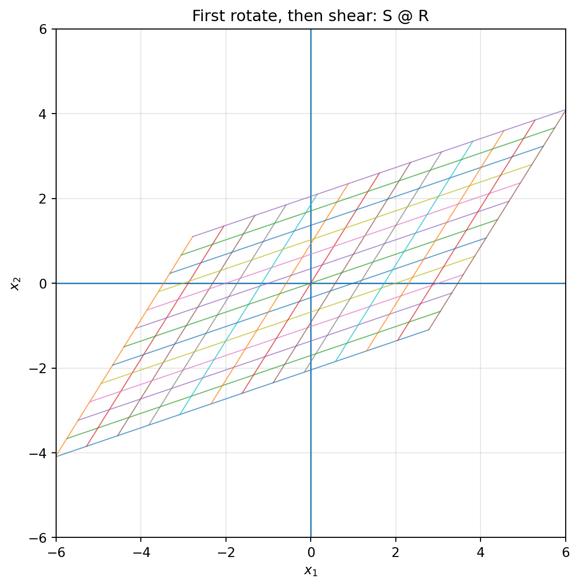
## 6.12 Composition: doing one transformation after another
Suppose we first apply $A$, then apply $B$. The final result is
$$
x \mapsto A x \mapsto B(Ax).
$$
This is
$$
B(Ax)=(BA)x.
$$
So composition of transformations corresponds to matrix multiplication.
::: {.callout-warning}
## Order matters
In general,
$$
BA\ne AB.
$$
Doing a rotation and then a shear is usually different from doing a shear and then a rotation.
:::
```{python}
theta = np.pi / 6
R = np.array([[np.cos(theta), -np.sin(theta)],
              [np.sin(theta),  np.cos(theta)]])
S = np.array([[1, 1.2],
              [0, 1]])

RS = R @ S
SR = S @ R

print("R @ S =\n", RS)
print("S @ R =\n", SR)

plot_grid(RS, title="First shear, then rotate: R @ S")
plot_grid(SR, title="First rotate, then shear: S @ R")
```
The notation can feel backward at first. In $(R S)x$, the matrix $S$ acts first, then $R$ acts second. This is because the vector is written on the right.
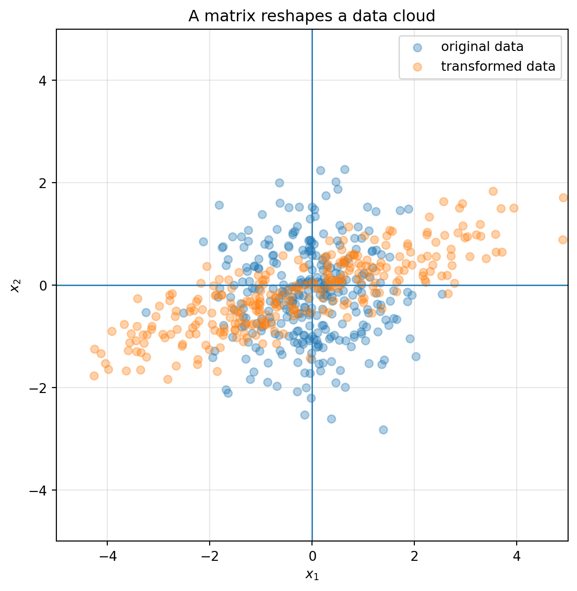
## 6.13 Transforming data clouds
Matrices do not only move ideal geometric shapes. They also move data.
A dataset with two numerical features can be represented as a cloud of points in $\mathbb R^2$. Applying a matrix transforms the entire data cloud.
```{python}
rng = np.random.default_rng(7)
X = rng.normal(size=(300, 2))

A = np.array([[2.0, 1.0],
              [0.4, 0.7]])
Y = transform_points(A, X)

fig, ax = plt.subplots(figsize=(7, 7))
draw_axes(ax, lim=5)
ax.scatter(X[:, 0], X[:, 1], alpha=0.35, label="original data")
ax.scatter(Y[:, 0], Y[:, 1], alpha=0.35, label="transformed data")
ax.set_title("A matrix reshapes a data cloud")
ax.legend()
plt.show()
```
This is why linear algebra is central in data science. A matrix can mix features, rotate coordinates, stretch important directions, compress weak directions, or collapse data into a lower-dimensional summary.
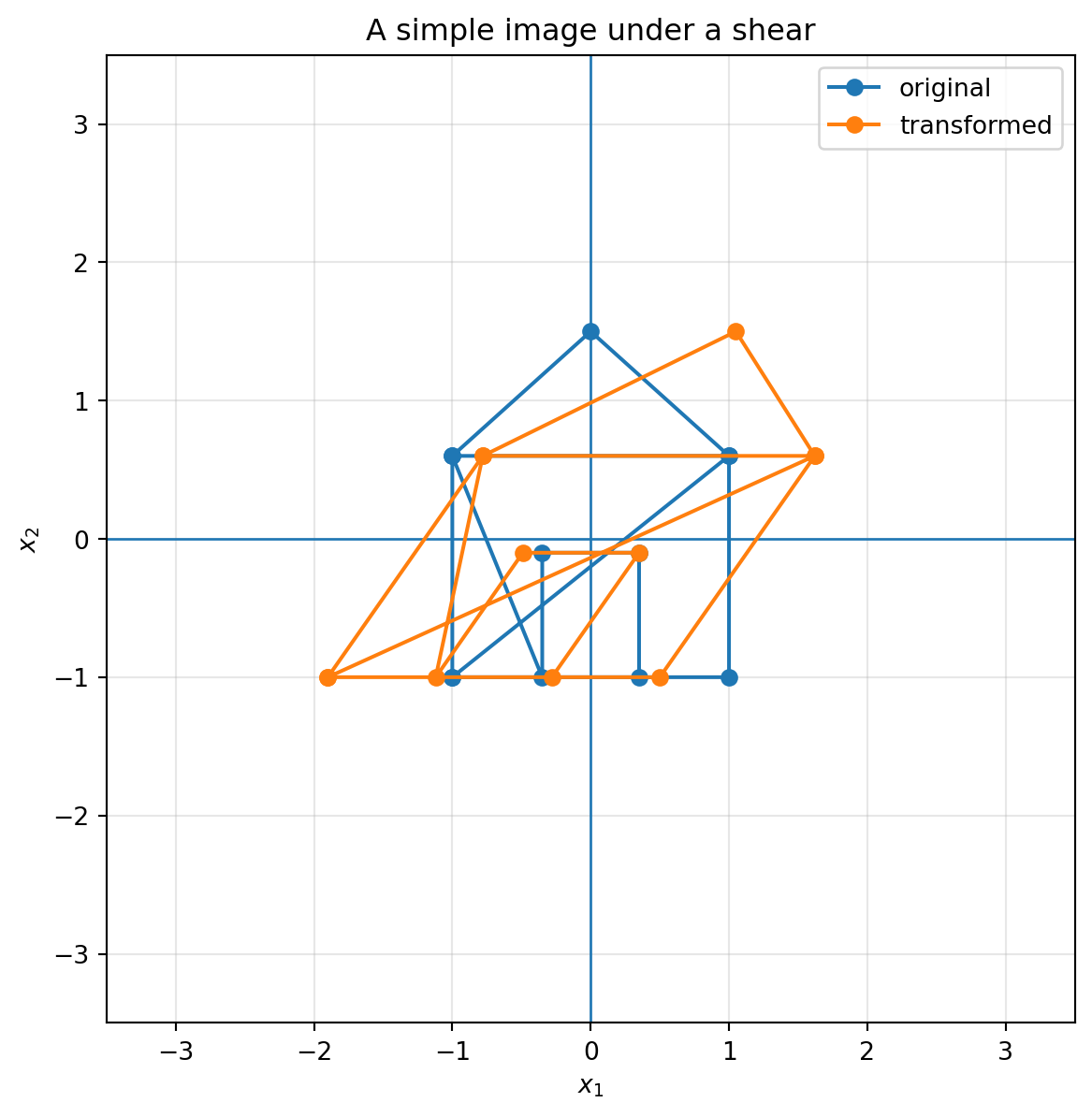
## 6.14 Image transformations
A grayscale image can be thought of as a matrix of pixel intensities. But the locations of pixels also live in the plane. If we apply a geometric matrix to pixel coordinates, we can rotate, shear, or scale an image.
Here is a simple point-picture made from coordinates. We transform the coordinates directly.
```{python}
# A small "house" drawing as points and line segments
house = np.array([
    [-1, -1], [1, -1], [1, 0.6], [0, 1.5], [-1, 0.6], [-1, -1],
    [1, 0.6], [-1, 0.6],
    [-0.35, -1], [-0.35, -0.1], [0.35, -0.1], [0.35, -1]
])

A = np.array([[1.2, 0.7],
              [0.0, 1.0]])

plot_shape(A, house, lim=3.5, title="A simple image under a shear")
```
Computer graphics uses these ideas constantly. Scaling, rotation, shear, reflection, camera transformations, and coordinate changes are all matrix operations.
## 6.15 A gallery of common $2\times 2$ transformations
| Transformation | Matrix | Geometric effect |
|---|---:|---|
| Identity | $\begin{bmatrix}1&0\\0&1\end{bmatrix}$ | Leaves everything unchanged |
| Horizontal stretch | $\begin{bmatrix}s&0\\0&1\end{bmatrix}$ | Multiplies horizontal coordinates by $s$ |
| Vertical stretch | $\begin{bmatrix}1&0\\0&s\end{bmatrix}$ | Multiplies vertical coordinates by $s$ |
| Reflection across $x_1$-axis | $\begin{bmatrix}1&0\\0&-1\end{bmatrix}$ | Flips up/down |
| Reflection across $x_2$-axis | $\begin{bmatrix}-1&0\\0&1\end{bmatrix}$ | Flips left/right |
| Horizontal shear | $\begin{bmatrix}1&k\\0&1\end{bmatrix}$ | Slides points horizontally depending on height |
| Vertical shear | $\begin{bmatrix}1&0\\k&1\end{bmatrix}$ | Slides points vertically depending on horizontal position |
| Rotation | $\begin{bmatrix}\cos\theta&-\sin\theta\\\sin\theta&\cos\theta\end{bmatrix}$ | Turns the plane by angle $\theta$ |
| Collapse | columns dependent | Flattens area to a line or point |
## 6.16 Worked examples
### Example 1: identify the transformation
Let
$$
A=
\begin{bmatrix}
3 & 0\\
0 & 1
\end{bmatrix}.
$$
Then
$$
Ae_1=\begin{bmatrix}3\\0\end{bmatrix},
\qquad
Ae_2=\begin{bmatrix}0\\1\end{bmatrix}.
$$
So the horizontal direction is stretched by a factor of $3$, while the vertical direction stays the same. This is a horizontal stretch.
### Example 2: identify a shear
Let
$$
A=
\begin{bmatrix}
1 & -2\\
0 & 1
\end{bmatrix}.
$$
Then
$$
Ae_1=e_1,
\qquad
Ae_2=-2e_1+e_2.
$$
The first basis vector stays fixed. The second basis vector slides left by two units. This is a horizontal shear.
### Example 3: compute area change
Let
$$
A=
\begin{bmatrix}
2 & 1\\
1 & 3
\end{bmatrix}.
$$
Then
$$
\det(A)=2\cdot 3-1\cdot 1=5.
$$
Every area is multiplied by $5$. The unit square becomes a parallelogram of area $5$.
### Example 4: check whether information is lost
Let
$$
A=
\begin{bmatrix}
2 & 4\\
1 & 2
\end{bmatrix}.
$$
The second column is twice the first. So the columns are dependent and
$$
\det(A)=2\cdot 2-4\cdot 1=0.
$$
The matrix collapses the plane onto a line. Information is lost.
## 6.17 Practice problems
### Problem 1
For each matrix, describe the transformation geometrically.
$$
A_1=\begin{bmatrix}2&0\\0&2\end{bmatrix},
\qquad
A_2=\begin{bmatrix}1&3\\0&1\end{bmatrix},
\qquad
A_3=\begin{bmatrix}0&-1\\1&0\end{bmatrix}.
$$
::: {.callout-tip collapse="true"}
## Solution
$A_1$ stretches all lengths by a factor of $2$.
$A_2$ is a horizontal shear with shear factor $3$.
$A_3$ is a rotation by $90^\circ$ counterclockwise.
:::
### Problem 2
Find the image of the unit square under
$$
A=\begin{bmatrix}
2 & 1\\
0 & 3
\end{bmatrix}.
$$
What is its area?
::: {.callout-tip collapse="true"}
## Solution
The corners of the unit square are
$$
0,\quad e_1,\quad e_1+e_2,\quad e_2.
$$
Their images are
$$
0,
\quad
Ae_1=\begin{bmatrix}2\\0\end{bmatrix},
\quad
Ae_1+Ae_2=\begin{bmatrix}3\\3\end{bmatrix},
\quad
Ae_2=\begin{bmatrix}1\\3\end{bmatrix}.
$$
The area is
$$
|\det(A)|=|2\cdot 3-1\cdot 0|=6.
$$
:::
### Problem 3
Let
$$
A=\begin{bmatrix}
1 & 2\\
2 & 4
\end{bmatrix}.
$$
Explain geometrically why $A$ cannot have an inverse.
::: {.callout-tip collapse="true"}
## Solution
The two columns are dependent because the second column is twice the first. Therefore the unit square collapses to a line segment. Since many input points land on the same output line, the original point cannot be recovered uniquely. Hence $A$ has no inverse.
:::
### Problem 4
Let
$$
R=\begin{bmatrix}
0 & -1\\
1 & 0
\end{bmatrix},
\qquad
S=\begin{bmatrix}
1 & 2\\
0 & 1
\end{bmatrix}.
$$
Compute $RS$ and $SR$. Are they equal?
::: {.callout-tip collapse="true"}
## Solution
$$
RS=
\begin{bmatrix}
0 & -1\\
1 & 0
\end{bmatrix}
\begin{bmatrix}
1 & 2\\
0 & 1
\end{bmatrix}
=
\begin{bmatrix}
0 & -1\\
1 & 2
\end{bmatrix}.
$$
$$
SR=
\begin{bmatrix}
1 & 2\\
0 & 1
\end{bmatrix}
\begin{bmatrix}
0 & -1\\
1 & 0
\end{bmatrix}
=
\begin{bmatrix}
2 & -1\\
1 & 0
\end{bmatrix}.
$$
They are not equal. The order of transformations matters.
:::
## 6.18 Challenge questions
1. Can a matrix preserve area but still change angles? Give an example.
2. Can a matrix preserve lengths but reverse orientation? Give an example.
3. What does the grid look like when $\det(A)$ is very close to zero but not exactly zero?
4. How can you tell from the columns of $A$ whether the matrix is likely to strongly stretch one direction?
5. Why does a rotation matrix have determinant $1$?
::: {.callout-tip collapse="true"}
## Discussion
1. Yes. A shear such as $\begin{bmatrix}1&1\\0&1\end{bmatrix}$ has determinant $1$ but changes angles.
2. Yes. A reflection preserves lengths but has determinant $-1$.
3. The grid becomes very thin. The plane is almost collapsed onto a line.
4. If the columns are long or nearly point in the same direction, the matrix may stretch some directions strongly and squeeze others.
5. A rotation preserves area and orientation, so its determinant is $1$.
:::
## 6.19 AI companion activities
Use an AI assistant as a mathematical conversation partner. Do not only ask for answers. Ask for explanations, counterexamples, and visual intuition.
### Prompt 1: explain the columns
> I am learning linear algebra. Explain why the columns of a $2\times 2$ matrix tell where the standard basis vectors go. Give a geometric example and a numerical example.
### Prompt 2: transformation detective
> Create five $2\times 2$ matrices. For each one, ask me to identify whether it is a stretch, reflection, shear, rotation, collapse, or combination. After I answer, explain the geometry.
### Prompt 3: determinant intuition
> Explain determinant as signed area change. Use the unit square, the column parallelogram, and orientation. Avoid starting with the formula.
### Prompt 4: Python visualization
> Write Python code that plots a grid before and after applying a $2\times 2$ matrix. Include a rotation, shear, reflection, and collapse example.
## 6.20 Chapter summary
A matrix is a machine, but in this chapter we learned to see the machine geometrically.
- A $2\times 2$ matrix transforms the whole plane.
- The first column is $Ae_1$ and the second column is $Ae_2$.
- A square usually becomes a parallelogram.
- Diagonal matrices stretch or squeeze coordinate directions.
- Reflection flips orientation.
- Shear slants space.
- Rotation turns space while preserving lengths, angles, and areas.
- The determinant measures signed area change.
- A zero determinant means space collapses and information is lost.
- Matrix multiplication represents composition of transformations.
The next chapters will build on this geometry. Once we can see matrices as transformations, we can understand solving equations, losing information, measuring distances, projecting data, finding stable directions, and decomposing complex systems.