---
title: "Chapter 2: Vectors — Numbers with Meaning"
subtitle: "Arrows, points, features, states, and stories encoded as coordinates"
format:
html:
toc: true
toc-depth: 3
number-sections: true
code-fold: true
code-tools: true
jupyter: python3
---
## Opening Story: The Same Numbers, Different Worlds
Imagine that you see the vector
$$
x=
\begin{bmatrix}
3\\
4
\end{bmatrix}.
$$
What does it mean?
At first, it looks like only two numbers stacked vertically. But those two numbers could describe many different things:
- walk $3$ blocks east and $4$ blocks north;
- move from the origin to the point $(3,4)$;
- a robot's velocity: $3$ meters per second horizontally and $4$ vertically;
- a customer buying $3$ coffees and $4$ sandwiches;
- a small image patch with two brightness values;
- a document containing $3$ occurrences of one word and $4$ occurrences of another.
The numbers are the same. The meaning changes with the coordinate system and the story attached to the coordinates.
This is one of the first major ideas in linear algebra:
::: {.callout-important}
A vector is not merely a list of numbers.
A vector is a list of numbers whose positions have meaning.
:::
Chapter 1 introduced the idea that the world can be translated into numbers. Chapter 2 begins the grammar of that translation. We learn how vectors behave, how they can be drawn, how they can describe data, and how basic vector operations become meaningful actions: combining, scaling, reversing, comparing, and measuring.
## Learning Goals
By the end of this chapter, you should be able to:
1. Interpret a vector as a point, arrow, movement, feature list, signal, or state.
2. Explain why order and coordinate meaning matter.
3. Add, subtract, and scale vectors by hand and in Python.
4. Interpret vector operations in geometric and data contexts.
5. Compute vector length and distance.
6. Understand why scaling features changes distances.
7. Work with vectors in dimensions too high to draw.
8. Use Python to visualize vectors and explore high-dimensional behavior.
## 2.1 From Numbers to Coordinates
A single number can measure one thing: temperature, price, age, distance, brightness, or speed.
A vector measures several things at once.
For example, a simple weather state might be encoded as
$$
w=
\begin{bmatrix}
72\\
65\\
12\\
1015\\
40\\
38
\end{bmatrix}.
$$
This vector becomes meaningful only when we know what each coordinate means:
$$
\begin{bmatrix}
\text{temperature in Fahrenheit}\\
\text{humidity percentage}\\
\text{wind speed in mph}\\
\text{air pressure in hPa}\\
\text{chance of rain percentage}\\
\text{air quality index}
\end{bmatrix}.
$$
The coordinate positions are part of the meaning. If we accidentally switch humidity and wind speed, the vector no longer describes the same weather.
::: {.callout-warning}
## Coordinate order matters
The vectors
$$
\begin{bmatrix}72\\65\\12\end{bmatrix}
\quad \text{and} \quad
\begin{bmatrix}72\\12\\65\end{bmatrix}
$$
contain the same three numbers, but they do not represent the same object if the second coordinate has a different meaning.
:::
## 2.2 Definition of a Vector
A vector in $\mathbb{R}^n$ is an ordered list of $n$ real numbers.
$$
x=
\begin{bmatrix}
x_1\\
x_2\\
\vdots\\
x_n
\end{bmatrix}
\in \mathbb{R}^n.
$$
The numbers $x_1,x_2,\ldots,x_n$ are called **coordinates** or **components**.
::: {.callout-important}
## Definition: Vector
A vector in $\mathbb{R}^n$ is an ordered list of $n$ real numbers:
$$
x=\begin{bmatrix}x_1\\x_2\\\vdots\\x_n\end{bmatrix}.
$$
The number $n$ is the **dimension** of the vector.
:::
Examples:
$$
\begin{bmatrix}3\\2\end{bmatrix}\in\mathbb{R}^2,
\qquad
\begin{bmatrix}4\\-1\\7\end{bmatrix}\in\mathbb{R}^3,
\qquad
\begin{bmatrix}x_1\\x_2\\\cdots\\x_{1000}\end{bmatrix}\in\mathbb{R}^{1000}.
$$
A vector in $\mathbb{R}^{1000}$ cannot be drawn on paper, but it can still be computed, compared, transformed, and used to model real objects.
## 2.3 Three Views of the Same Vector
The vector
$$
v=\begin{bmatrix}3\\2\end{bmatrix}
$$
has several useful interpretations.
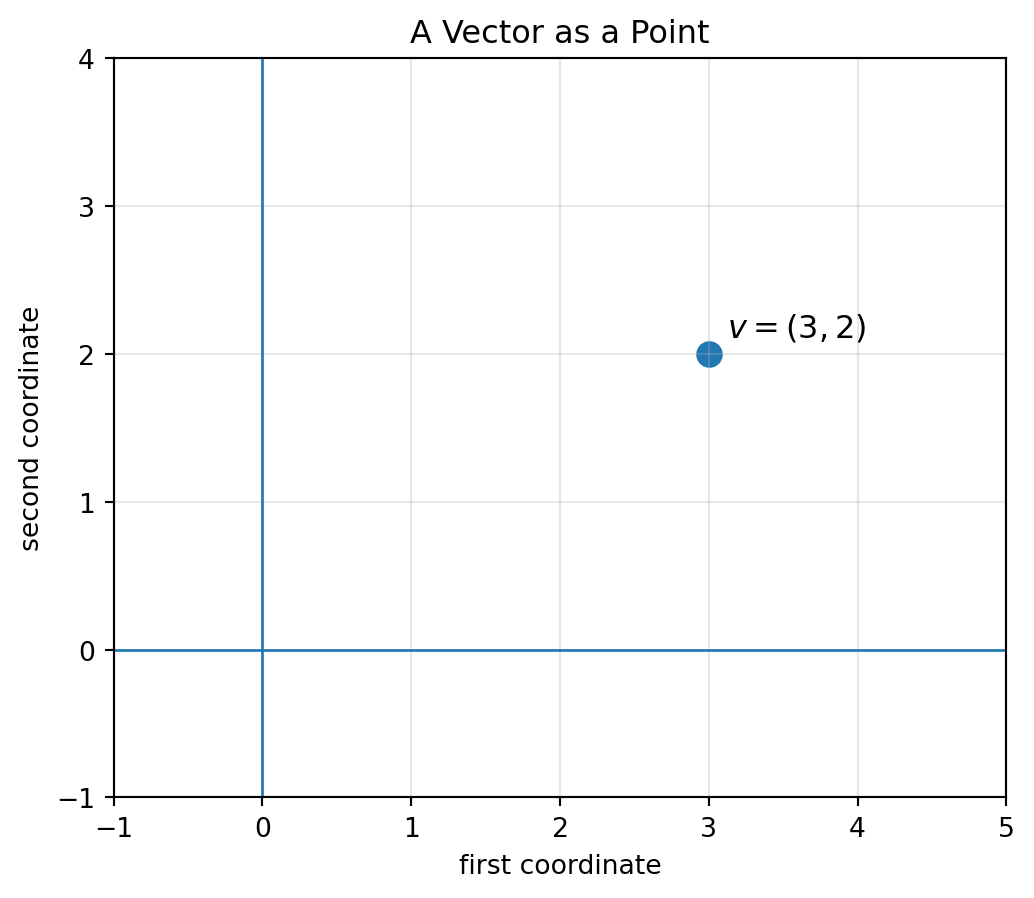
### View 1: A vector as a point
As a point, $v$ represents the location $(3,2)$.
```{python}
import numpy as np
import matplotlib.pyplot as plt

v = np.array([3, 2])

plt.figure(figsize=(6, 5))
plt.scatter(v[0], v[1], s=80)
plt.text(v[0] + 0.12, v[1] + 0.12, "$v=(3,2)$", fontsize=12)
plt.axhline(0, linewidth=1)
plt.axvline(0, linewidth=1)
plt.xlim(-1, 5)
plt.ylim(-1, 4)
plt.xlabel("first coordinate")
plt.ylabel("second coordinate")
plt.title("A Vector as a Point")
plt.grid(True, alpha=0.3)
plt.show()
```
When vectors represent data, this point view is natural. A person, song, city, image, or document can become a point in feature space.
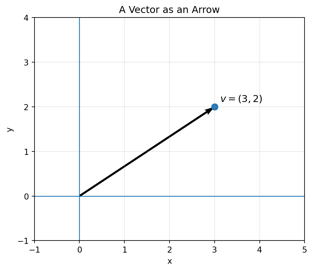
### View 2: A vector as an arrow
As an arrow, $v$ describes movement: start at $(0,0)$ and move $3$ units horizontally and $2$ units vertically.
```{python}
plt.figure(figsize=(6, 5))
plt.quiver(0, 0, v[0], v[1], angles="xy", scale_units="xy", scale=1)
plt.scatter(v[0], v[1], s=60)
plt.text(v[0] + 0.12, v[1] + 0.12, "$v=(3,2)$", fontsize=12)
plt.axhline(0, linewidth=1)
plt.axvline(0, linewidth=1)
plt.xlim(-1, 5)
plt.ylim(-1, 4)
plt.xlabel("x")
plt.ylabel("y")
plt.title("A Vector as an Arrow")
plt.grid(True, alpha=0.3)
plt.show()
```
When vectors represent motion, force, velocity, or direction, the arrow view is natural.
### View 3: A vector as a feature list
A movie might be represented as
$$
m=
\begin{bmatrix}
8.5\\
120\\
0.7\\
0.2\\
0.9
\end{bmatrix},
\qquad
\begin{bmatrix}
\text{average rating}\\
\text{length in minutes}\\
\text{action score}\\
\text{comedy score}\\
\text{drama score}
\end{bmatrix}.
$$
This vector is not mainly an arrow in physical space. It is a compact description of an object.
::: {.callout-note}
## One mathematical object, many interpretations
A vector may be a point, an arrow, a movement, a signal, a list of features, a state of a system, or a row of data. The algebra is the same, but the interpretation depends on the story.
:::
## 2.4 A Vector Space Preview
For now, we work mainly with vectors in $\mathbb{R}^n$. Later, we will use a more general idea called a **vector space**. The core behavior is already visible here:
- we can add two vectors of the same dimension;
- we can multiply a vector by a scalar;
- the result is still a vector of the same dimension.
This simple closure property is the beginning of linear algebra.
::: {.callout-tip}
## Informal principle
A collection of objects begins to behave like a vector space when you can combine objects and scale them while staying inside the same kind of object.
:::
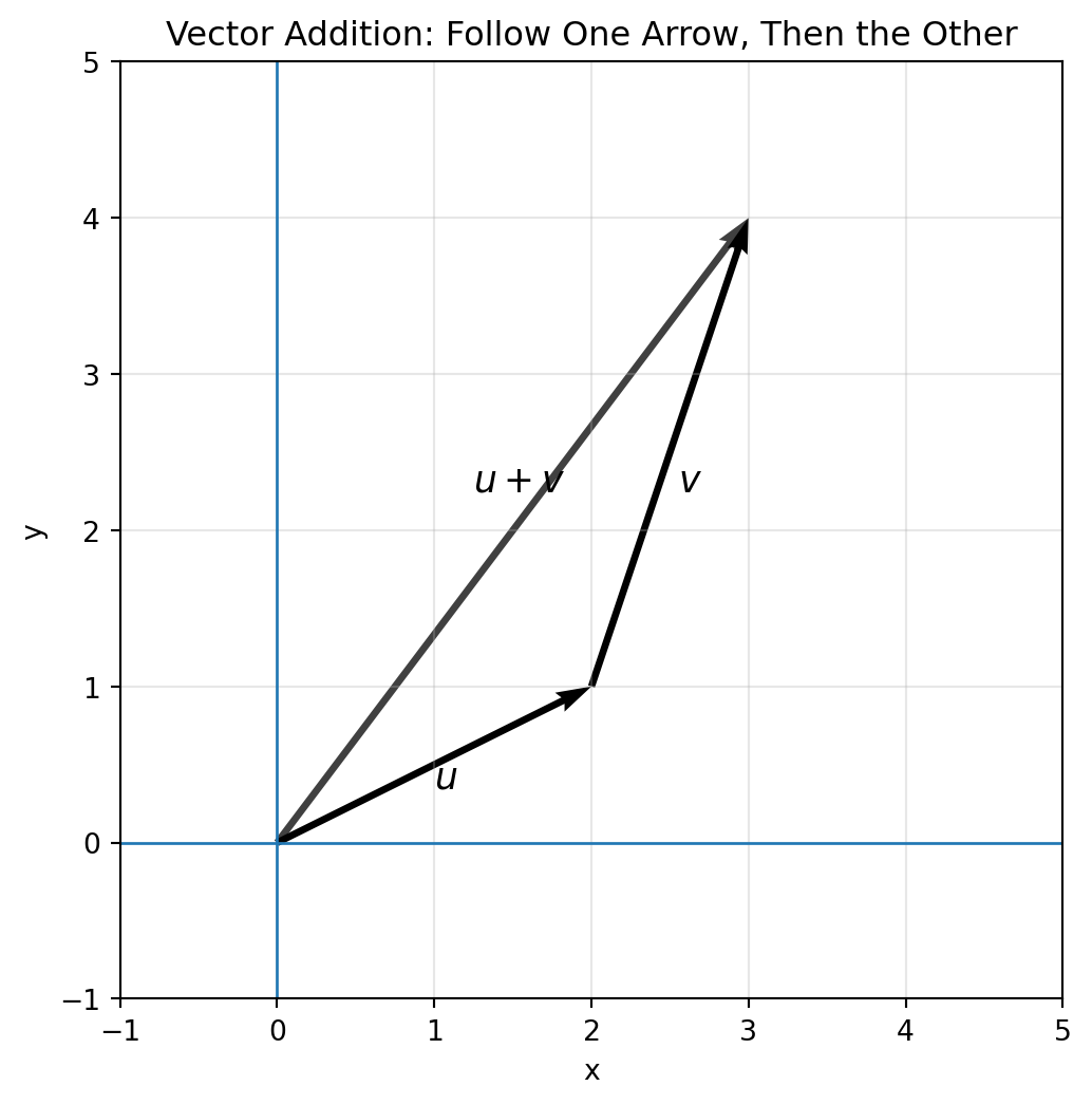
## 2.5 Vector Addition: Combining Movements
Let
$$
u=\begin{bmatrix}2\\1\end{bmatrix},
\qquad
v=\begin{bmatrix}1\\3\end{bmatrix}.
$$
Then
$$
u+v=
\begin{bmatrix}2\\1\end{bmatrix}+
\begin{bmatrix}1\\3\end{bmatrix}
=
\begin{bmatrix}3\\4\end{bmatrix}.
$$
::: {.callout-important}
## Definition: Vector addition
If
$$
u=\begin{bmatrix}u_1\\u_2\\\vdots\\u_n\end{bmatrix},
\qquad
v=\begin{bmatrix}v_1\\v_2\\\vdots\\v_n\end{bmatrix},
$$
then
$$
u+v=
\begin{bmatrix}u_1+v_1\\u_2+v_2\\\vdots\\u_n+v_n\end{bmatrix}.
$$
:::
Geometrically, vector addition means doing one movement and then another.
```{python}
u = np.array([2, 1])
v = np.array([1, 3])
s = u + v

plt.figure(figsize=(6, 6))
plt.quiver(0, 0, u[0], u[1], angles="xy", scale_units="xy", scale=1)
plt.quiver(u[0], u[1], v[0], v[1], angles="xy", scale_units="xy", scale=1)
plt.quiver(0, 0, s[0], s[1], angles="xy", scale_units="xy", scale=1, alpha=0.75)
plt.text(1.0, 0.35, "$u$", fontsize=13)
plt.text(2.55, 2.25, "$v$", fontsize=13)
plt.text(1.25, 2.25, "$u+v$", fontsize=13)
plt.axhline(0, linewidth=1)
plt.axvline(0, linewidth=1)
plt.xlim(-1, 5)
plt.ylim(-1, 5)
plt.xlabel("x")
plt.ylabel("y")
plt.title("Vector Addition: Follow One Arrow, Then the Other")
plt.grid(True, alpha=0.3)
plt.show()
```
This picture is sometimes called the **tip-to-tail rule**.
## 2.6 Vector Addition: Combining Information
Suppose a student studies in two sessions. The coordinates mean
$$
\begin{bmatrix}
\text{algebra problems}\\
\text{geometry problems}\\
\text{word problems}
\end{bmatrix}.
$$
The first session is
$$
s_1=\begin{bmatrix}3\\2\\1\end{bmatrix},
$$
and the second session is
$$
s_2=\begin{bmatrix}2\\4\\3\end{bmatrix}.
$$
The total work is
$$
s_1+s_2=
\begin{bmatrix}5\\6\\4\end{bmatrix}.
$$
Here, addition means accumulation.
Other meanings of vector addition include:
| Context | What $u+v$ means |
|---|---|
| Movement | do movement $u$, then movement $v$ |
| Sales | combine sales from two days |
| Signals | add two sound waves or measurements |
| Text | combine word counts from two documents |
| Finance | combine holdings from two portfolios |
| Machine learning | combine feature effects or embeddings |
The formula is coordinate-wise addition, but the interpretation changes with the context.
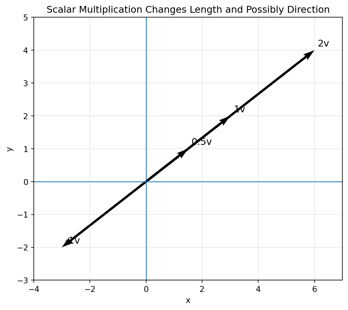
## 2.7 Scalar Multiplication: Changing Intensity
A **scalar** is a single number.
If
$$
v=\begin{bmatrix}3\\2\end{bmatrix},
$$
then
$$
2v=\begin{bmatrix}6\\4\end{bmatrix},
\qquad
\frac{1}{2}v=\begin{bmatrix}1.5\\1\end{bmatrix},
\qquad
-v=\begin{bmatrix}-3\\-2\end{bmatrix}.
$$
::: {.callout-important}
## Definition: Scalar multiplication
If $c$ is a scalar and
$$
v=\begin{bmatrix}v_1\\v_2\\\vdots\\v_n\end{bmatrix},
$$
then
$$
cv=\begin{bmatrix}cv_1\\cv_2\\\vdots\\cv_n\end{bmatrix}.
$$
:::
Geometrically:
- $2v$ points in the same direction as $v$, but is twice as long;
- $0.5v$ points in the same direction as $v$, but is half as long;
- $-v$ points in the opposite direction;
- $0v$ becomes the zero vector.
```{python}
v = np.array([3, 2])
scalars = [0.5, 1, 2, -1]

plt.figure(figsize=(7, 6))
for c in scalars:
    w = c * v
    plt.quiver(0, 0, w[0], w[1], angles="xy", scale_units="xy", scale=1)
    plt.text(w[0] + 0.12, w[1] + 0.12, f"{c}v", fontsize=12)
plt.axhline(0, linewidth=1)
plt.axvline(0, linewidth=1)
plt.xlim(-4, 7)
plt.ylim(-3, 5)
plt.xlabel("x")
plt.ylabel("y")
plt.title("Scalar Multiplication Changes Length and Possibly Direction")
plt.grid(True, alpha=0.3)
plt.show()
```
In a data story, scalar multiplication often means changing intensity. If $v$ is a shopping basket, then $2v$ is twice as much of everything. If $v$ is a sound wave, then $0.5v$ is a quieter version of the same wave.
## 2.8 The Zero Vector and Negative Vectors
The **zero vector** has all coordinates equal to zero:
$$
0=\begin{bmatrix}0\\0\\\vdots\\0\end{bmatrix}.
$$
It represents no movement, no signal, or no quantity, depending on context.
For every vector $v$,
$$
v+0=v.
$$
The **negative vector** $-v$ satisfies
$$
v+(-v)=0.
$$
If $v$ is a movement, then $-v$ undoes that movement.
::: {.callout-note}
## Algebra and meaning
The equation $v+(-v)=0$ is algebraic. But in a movement story, it says: move out, then move exactly back.
:::
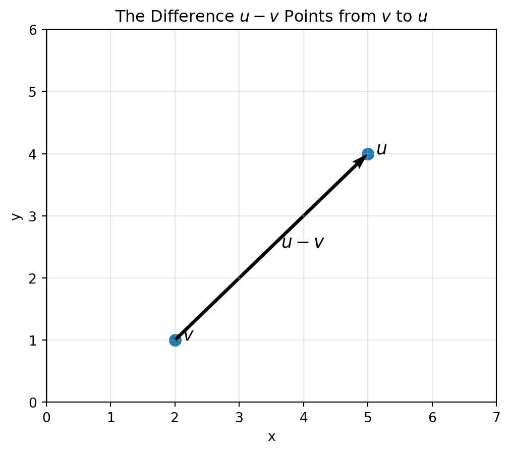
## 2.9 Vector Subtraction: Measuring Change
Subtraction is addition of the negative:
$$
u-v=u+(-v).
$$
For example,
$$
\begin{bmatrix}5\\4\end{bmatrix}
-
\begin{bmatrix}2\\1\end{bmatrix}
=
\begin{bmatrix}3\\3\end{bmatrix}.
$$
When $u$ and $v$ are points, $u-v$ is the arrow from $v$ to $u$.
```{python}
u = np.array([5, 4])
v = np.array([2, 1])
d = u - v

plt.figure(figsize=(6, 5))
plt.scatter([u[0], v[0]], [u[1], v[1]], s=70)
plt.text(u[0] + 0.12, u[1], "$u$", fontsize=13)
plt.text(v[0] + 0.12, v[1], "$v$", fontsize=13)
plt.quiver(v[0], v[1], d[0], d[1], angles="xy", scale_units="xy", scale=1)
plt.text(v[0] + d[0]/2 + 0.15, v[1] + d[1]/2, "$u-v$", fontsize=13)
plt.axhline(0, linewidth=1)
plt.axvline(0, linewidth=1)
plt.xlim(0, 7)
plt.ylim(0, 6)
plt.xlabel("x")
plt.ylabel("y")
plt.title("The Difference $u-v$ Points from $v$ to $u$")
plt.grid(True, alpha=0.3)
plt.show()
```
Subtraction is one of the first ways linear algebra measures change:
$$
\text{change} = \text{new state} - \text{old state}.
$$
## 2.10 Length: How Large Is a Vector?
The length of a vector is also called its **norm**.
For
$$
v=\begin{bmatrix}3\\4\end{bmatrix},
$$
the length is
$$
\|v\|=\sqrt{3^2+4^2}=5.
$$
::: {.callout-important}
## Definition: Euclidean norm
For
$$
v=\begin{bmatrix}v_1\\v_2\\\vdots\\v_n\end{bmatrix},
$$
the Euclidean norm is
$$
\|v\|=\sqrt{v_1^2+v_2^2+\cdots+v_n^2}.
$$
:::
In Python:
```{python}
v = np.array([3, 4])
np.linalg.norm(v)
```
The norm is a measure of size. But size has different meanings:
| Vector represents | Norm can measure |
|---|---|
| movement | distance traveled from the origin |
| force | magnitude of force |
| signal | energy or amplitude-like size |
| error vector | total error size |
| feature vector | overall scale of an object |
## 2.11 Distance: How Different Are Two Vectors?
If two vectors represent points, the distance between them is the length of their difference:
$$
\operatorname{dist}(u,v)=\|u-v\|.
$$
For example,
$$
u=\begin{bmatrix}5\\4\end{bmatrix},
\qquad
v=\begin{bmatrix}2\\1\end{bmatrix}.
$$
Then
$$
u-v=\begin{bmatrix}3\\3\end{bmatrix},
\qquad
\|u-v\|=\sqrt{3^2+3^2}=\sqrt{18}.
$$
```{python}
u = np.array([5, 4])
v = np.array([2, 1])
np.linalg.norm(u - v)
```
Distance is central in data science. If customers, documents, songs, or images are vectors, then distance becomes a way to measure similarity.
::: {.callout-warning}
## Distance depends on representation
If one coordinate is measured on a much larger scale than the others, it can dominate the distance calculation. This is why feature scaling is important.
:::
## 2.12 A Scaling Warning: When Units Take Over
Consider three restaurants represented by
$$
[\text{price level}, \text{distance in miles}, \text{rating}].
$$
```{python}
restaurants = {
    "A": np.array([2, 1.5, 4.6]),
    "B": np.array([3, 2.0, 4.8]),
    "C": np.array([1, 8.0, 4.2]),
}

for name1, x in restaurants.items():
    for name2, y in restaurants.items():
        if name1 < name2:
            print(name1, name2, np.linalg.norm(x-y))
```
The distance coordinate can dominate the calculation because miles vary more than ratings. If we measured distance in feet instead of miles, the distance coordinate would become even larger and dominate even more.
A common fix is to scale each feature before comparing vectors.
```{python}
X = np.vstack(list(restaurants.values()))
X_scaled = (X - X.mean(axis=0)) / X.std(axis=0)

for i, name1 in enumerate(restaurants):
    for j, name2 in enumerate(restaurants):
        if i < j:
            print(name1, name2, np.linalg.norm(X_scaled[i]-X_scaled[j]))
```
This is a first glimpse of a recurring lesson:
> Linear algebra can compute with vectors, but modeling choices decide what the computations mean.
## 2.13 Direction: Pattern Versus Size
Suppose two users rate four movies:
$$
a=\begin{bmatrix}5\\5\\1\\1\end{bmatrix},
\qquad
b=\begin{bmatrix}10\\10\\2\\2\end{bmatrix}.
$$
Then
$$
b=2a.
$$
User B gives ratings twice as large, but the pattern is the same. The two vectors point in the same direction.
In many applications, direction represents pattern, while length represents intensity.
::: {.callout-tip}
## Pattern versus intensity
Length measures size.
Direction measures pattern.
:::
Later we will use this idea to define cosine similarity, projections, principal component analysis, and recommendation systems.
## 2.14 Vectors in Higher Dimensions
The same operations work in high dimensions.
Let
$$
x=\begin{bmatrix}1\\2\\3\\4\\5\end{bmatrix},
\qquad
y=\begin{bmatrix}5\\4\\3\\2\\1\end{bmatrix}.
$$
Then
$$
x+y=\begin{bmatrix}6\\6\\6\\6\\6\end{bmatrix},
\qquad
x-y=\begin{bmatrix}-4\\-2\\0\\2\\4\end{bmatrix}.
$$
We cannot draw five dimensions faithfully, but computation does not care. A vector with $1000$ coordinates is still an ordered list. The rules remain coordinate-wise.
```{python}
x = np.arange(1, 1001)
y = np.arange(1000, 0, -1)

print("dimension of x:", x.shape[0])
print("first five entries of x+y:", (x+y)[:5])
print("norm of x:", np.linalg.norm(x))
print("distance between x and y:", np.linalg.norm(x-y))
```
Modern data often lives in high dimensions:
| Object | Possible vector dimension |
|---|---:|
| grayscale $28\times 28$ image | $784$ |
| color $224\times 224$ image | $150{,}528$ |
| bag-of-words document | $10{,}000$ or more |
| user preference vector | thousands or millions |
| neural network hidden state | hundreds to thousands |
Linear algebra is the language that lets us reason in spaces too large to visualize directly.
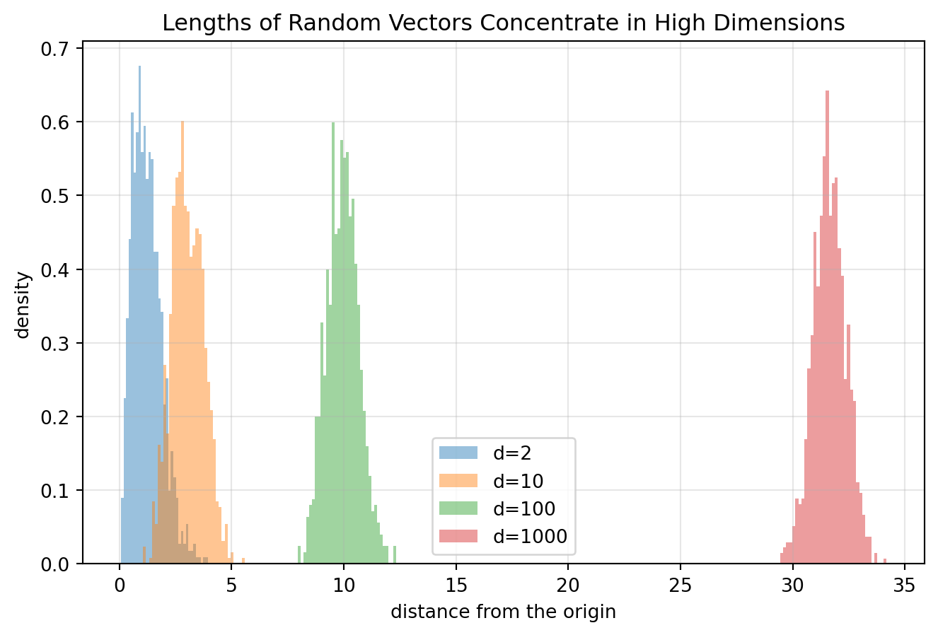
## 2.15 A High-Dimensional Surprise
In two dimensions, random points can be close or far in a familiar way. In high dimensions, distances behave differently.
The following simulation draws random points in dimensions $2$, $10$, $100$, and $1000$ and compares their distances from the origin.
```{python}
np.random.seed(7)

dims = [2, 10, 100, 1000]
num_points = 1000

plt.figure(figsize=(8, 5))
for d in dims:
    X = np.random.randn(num_points, d)
    lengths = np.linalg.norm(X, axis=1)
    plt.hist(lengths, bins=35, alpha=0.45, density=True, label=f"d={d}")

plt.xlabel("distance from the origin")
plt.ylabel("density")
plt.title("Lengths of Random Vectors Concentrate in High Dimensions")
plt.legend()
plt.grid(True, alpha=0.3)
plt.show()
```
In high dimensions, random lengths tend to concentrate around a typical value. This phenomenon will return later when we study data clouds, PCA, machine learning, and the geometry of high-dimensional spaces.
## 2.16 Mini-Project: A Tiny Recommendation Story
Suppose a user preference vector has coordinates
$$
[\text{action},\text{comedy},\text{drama},\text{romance},\text{sci-fi}].
$$
A user is represented by
$$
u=\begin{bmatrix}0.9\\0.2\\0.4\\0.1\\0.8\end{bmatrix}.
$$
Three movies are represented by
$$
m_1=\begin{bmatrix}0.8\\0.1\\0.3\\0.1\\0.9\end{bmatrix},\quad
m_2=\begin{bmatrix}0.1\\0.9\\0.4\\0.7\\0.1\end{bmatrix},\quad
m_3=\begin{bmatrix}0.4\\0.3\\0.9\\0.6\\0.2\end{bmatrix}.
$$
Which movie is closest to the user?
```{python}
user = np.array([0.9, 0.2, 0.4, 0.1, 0.8])
movies = {
    "Space Chase": np.array([0.8, 0.1, 0.3, 0.1, 0.9]),
    "Laugh & Love": np.array([0.1, 0.9, 0.4, 0.7, 0.1]),
    "Quiet Memory": np.array([0.4, 0.3, 0.9, 0.6, 0.2]),
}

for title, vec in movies.items():
    print(title, np.linalg.norm(user - vec))
```
This is a simple version of a recommendation idea: represent objects and users as vectors, then compare them.
## 2.17 What Can Go Wrong?
Vectors are powerful, but they are not magic. A vector representation can fail if:
1. important features are missing;
2. coordinates use incompatible units;
3. features are scaled poorly;
4. the order of coordinates is inconsistent;
5. distance is not the right measure of similarity;
6. the vector hides important qualitative information.
Linear algebra gives us a language. Modeling asks whether we are speaking the right language for the problem.
## 2.18 Concept Summary
| Concept | Formula | Meaning |
|---|---|---|
| vector | $x=[x_1,\ldots,x_n]^T$ | numbers with coordinate meaning |
| addition | $u+v$ | combine coordinate by coordinate |
| scalar multiplication | $cv$ | scale every coordinate by $c$ |
| negative vector | $-v$ | reverse direction or undo quantity |
| subtraction | $u-v$ | change from $v$ to $u$ |
| norm | $\|v\|$ | length or size |
| distance | $\|u-v\|$ | difference between vectors |
| direction | pattern | relative coordinate structure |
The most important idea is that algebraic operations become meaningful only after we interpret the coordinates.
## 2.19 Practice Problems
### Problem 1: Basic operations
Let
$$
u=\begin{bmatrix}2\\5\end{bmatrix},
\qquad
v=\begin{bmatrix}3\\-1\end{bmatrix}.
$$
Compute $u+v$, $u-v$, $2u$, $-v$, and $3u-2v$.
::: {.callout-tip collapse="true"}
## Solution
$$
u+v=\begin{bmatrix}5\\4\end{bmatrix},
\qquad
u-v=\begin{bmatrix}-1\\6\end{bmatrix},
\qquad
2u=\begin{bmatrix}4\\10\end{bmatrix},
\qquad
-v=\begin{bmatrix}-3\\1\end{bmatrix}.
$$
Also,
$$
3u-2v=\begin{bmatrix}6\\15\end{bmatrix}-\begin{bmatrix}6\\-2\end{bmatrix}=\begin{bmatrix}0\\17\end{bmatrix}.
$$
:::
### Problem 2: Length and distance
Let
$$
x=\begin{bmatrix}1\\2\\3\end{bmatrix},
\qquad
y=\begin{bmatrix}4\\0\\-2\end{bmatrix}.
$$
Compute $x+y$, $y-x$, $\|x\|$, and $\|x-y\|$.
::: {.callout-tip collapse="true"}
## Solution
$$
x+y=\begin{bmatrix}5\\2\\1\end{bmatrix},
\qquad
y-x=\begin{bmatrix}3\\-2\\-5\end{bmatrix}.
$$
$$
\|x\|=\sqrt{1^2+2^2+3^2}=\sqrt{14}.
$$
$$
x-y=\begin{bmatrix}-3\\2\\5\end{bmatrix},
\qquad
\|x-y\|=\sqrt{(-3)^2+2^2+5^2}=\sqrt{38}.
$$
:::
### Problem 3: Meaning of a change vector
A patient is represented by
$$
p=\begin{bmatrix}70\\160\\25\end{bmatrix},
$$
where the coordinates are height in inches, weight in pounds, and age in years. What does
$$
p+
\begin{bmatrix}0\\5\\1\end{bmatrix}
$$
represent?
::: {.callout-tip collapse="true"}
## Solution
The new vector is
$$
\begin{bmatrix}70\\165\\26\end{bmatrix}.
$$
It represents the same height, $5$ more pounds, and $1$ year older. Whether this is a meaningful model depends on the context: age changes predictably, but weight and height may require real measurement.
:::
### Problem 4: Modeling interpretation
Give three interpretations of
$$
\begin{bmatrix}3\\4\end{bmatrix}
$$
where vector addition has different meanings in each interpretation.
::: {.callout-tip collapse="true"}
## Sample answer
1. Movement: $3$ steps east and $4$ steps north. Addition means doing two movements in sequence.
2. Shopping: $3$ coffees and $4$ sandwiches. Addition means combining purchases.
3. Word counts: $3$ counts of word A and $4$ counts of word B. Addition means combining documents.
:::
### Problem 5: Scaling issue
A data vector uses coordinates $[\text{age in years},\text{income in dollars}]$. Explain why Euclidean distance may be dominated by income.
::: {.callout-tip collapse="true"}
## Solution
Income may vary by tens of thousands, while age may vary by tens. In the Euclidean distance formula, the income difference will usually be much larger, so it dominates the total distance. Scaling or standardization is usually needed before comparing such vectors.
:::
## 2.20 Python Practice
### Exercise 1
Create two vectors in $\mathbb{R}^4$ and compute their sum, difference, and scalar multiples.
```{python}
u = np.array([2, -1, 0, 5])
v = np.array([3, 4, -2, 1])

print("u+v =", u+v)
print("u-v =", u-v)
print("3u =", 3*u)
print("-2v =", -2*v)
```
### Exercise 2
Compute the lengths of ten random vectors in $\mathbb{R}^{20}$.
```{python}
np.random.seed(2)
X = np.random.randn(10, 20)
lengths = np.linalg.norm(X, axis=1)
lengths
```
### Exercise 3
Create five song vectors using the features
$$
[\text{tempo},\text{energy},\text{danceability},\text{acousticness}].
$$
Then compute which two songs are closest.
```{python}
songs = np.array([
    [120, 0.80, 0.75, 0.10],
    [118, 0.82, 0.78, 0.12],
    [75, 0.30, 0.40, 0.85],
    [140, 0.95, 0.65, 0.05],
    [90, 0.50, 0.55, 0.60],
])

# Standardize before comparing because tempo is on a different scale.
songs_scaled = (songs - songs.mean(axis=0)) / songs.std(axis=0)

best_pair = None
best_distance = float("inf")

for i in range(len(songs)):
    for j in range(i+1, len(songs)):
        d = np.linalg.norm(songs_scaled[i] - songs_scaled[j])
        if d < best_distance:
            best_distance = d
            best_pair = (i, j)

best_pair, best_distance
```
## 2.21 AI Companion Activities
### Activity 1: Explain the same vector in five worlds
Ask an AI tool:
> Give five real-world interpretations of the vector $[3,4]$. For each interpretation, explain what vector addition and scalar multiplication would mean.
Then choose the interpretation where the algebra feels most natural.
### Activity 2: Critique a vector representation
Ask:
> Suppose a student is represented by $[\text{GPA},\text{number of courses},\text{hours studied per week}]$. What are the strengths and weaknesses of this vector representation?
Then improve the representation by adding or changing features.
### Activity 3: Create a high-dimensional example
Ask:
> Create a realistic example of a 100-dimensional vector. What do the coordinates mean? What would distance mean?
Check whether the answer explains the coordinate meanings clearly.
### Activity 4: Prompt for precision
Ask:
> Explain why a vector is more than a list of numbers, but keep the explanation mathematically precise.
Revise the answer until it uses both intuition and correct mathematical language.
## 2.22 Reflection Questions
1. Why does coordinate order matter?
2. What is the difference between a vector as a point and a vector as an arrow?
3. Give an example where vector addition means accumulation.
4. Give an example where vector addition means movement.
5. What does scalar multiplication by a negative number do?
6. Why is $u-v$ the arrow from $v$ to $u$?
7. What does $\|v\|$ measure?
8. Why does feature scaling matter before computing distances?
9. In what kind of problem might direction matter more than length?
10. What is one danger of translating a real object into a vector?
## 2.23 Chapter Closing: The First Grammar Rule
In this chapter, vectors became more than lists of numbers. They became a language.
A vector can describe a point, an arrow, a motion, a signal, a customer, a document, a song, a weather state, or a hidden state inside an AI model. The same operations keep appearing:
- add vectors to combine information;
- scale vectors to change intensity;
- subtract vectors to measure change;
- take norms to measure size;
- take distances to compare objects.
These are simple rules, but they are the first grammar rules of linear algebra.
In the next chapter, we take a major step: instead of adding only two vectors, we learn how to build new vectors by combining many vectors with different weights. That idea is called a **linear combination**, and it leads directly to span, basis, dimension, and the geometry of possibility.