Best approximation, residuals, least squares, and the geometry of being as close as possible
11.1 Opening Story: The Shadow That Loses the Least
Imagine a complicated object in three-dimensional space: a person, a building, a cloud, a moving airplane. Now shine a light on it and look at the shadow on a wall. The shadow is simpler than the original object. It has fewer dimensions. It has lost information. Yet it is not random. It is the version of the object that remains after we keep only the part that can be seen from a chosen direction.
Projection is the mathematical version of this idea. A projection takes a vector and replaces it by its best shadow on a simpler space: a line, a plane, or a subspace.
The word best is crucial. Projection is not merely throwing information away. It is throwing information away in the most controlled possible way. Among all vectors in the simpler space, the projection is the one closest to the original vector.
This chapter introduces one of the most important principles in applied linear algebra:
When we cannot represent something exactly, we often represent it by the closest thing we can build.
That closest thing is a projection. The leftover part is called the residual. The magic fact is that the residual is perpendicular to the space of approximation.
In the language of this book:
Projection is the best shadow, and orthogonality explains why it is best.
This idea becomes the heart of least squares, regression, signal approximation, PCA, image compression, recommendation systems, and many algorithms in machine learning.
11.2 Learning Goals
By the end of this chapter, you should be able to:
Explain projection as a closest-point problem.
Compute the projection of a vector onto a line.
Interpret the projection coefficient as the amount of one direction inside another vector.
Explain why the residual is orthogonal to the approximation space.
Use projection to decompose a vector into a visible part and an invisible error part.
Compute projections onto subspaces with orthonormal bases.
Understand the matrix formula \(P = QQ^T\) for orthogonal projection.
Understand the least-squares formula \(\hat{x}=(A^TA)^{-1}A^Tb\) when the columns of \(A\) are independent.
Use Python to visualize projections, residuals, and least-squares fits.
Connect projection to data science, regression, signal processing, and machine learning.
11.3 11.1 Projection as a Closest-Point Problem
Let \(y\) be a vector in \(\mathbb{R}^n\). Let \(S\) be a subspace of \(\mathbb{R}^n\).
The projection of \(y\) onto \(S\) is the vector \(\hat{y}\) in \(S\) that is closest to \(y\):
\[
\hat{y}=\operatorname{proj}_S(y).
\]
This means that \(\hat{y}\) solves the optimization problem
\[
\hat{y}=\arg\min_{z\in S}\|y-z\|.
\]
The vector
\[
r=y-\hat{y}
\]
is called the residual or error vector. It measures what remains after the best approximation has been made.
The fundamental geometry is:
\[
y=\hat{y}+r,
\]
where
\[
\hat{y}\in S
\qquad \text{and} \qquad
r\perp S.
\]
This says:
\(\hat{y}\) is the part of \(y\) that lives in the subspace \(S\).
\(r\) is the part of \(y\) that cannot be explained by \(S\).
The explained part and unexplained part are perpendicular.
This is the main picture of the chapter.
TipThe projection principle
The best approximation from a subspace is found when the error is perpendicular to every direction inside that subspace.
11.4 11.2 Projection onto a Line
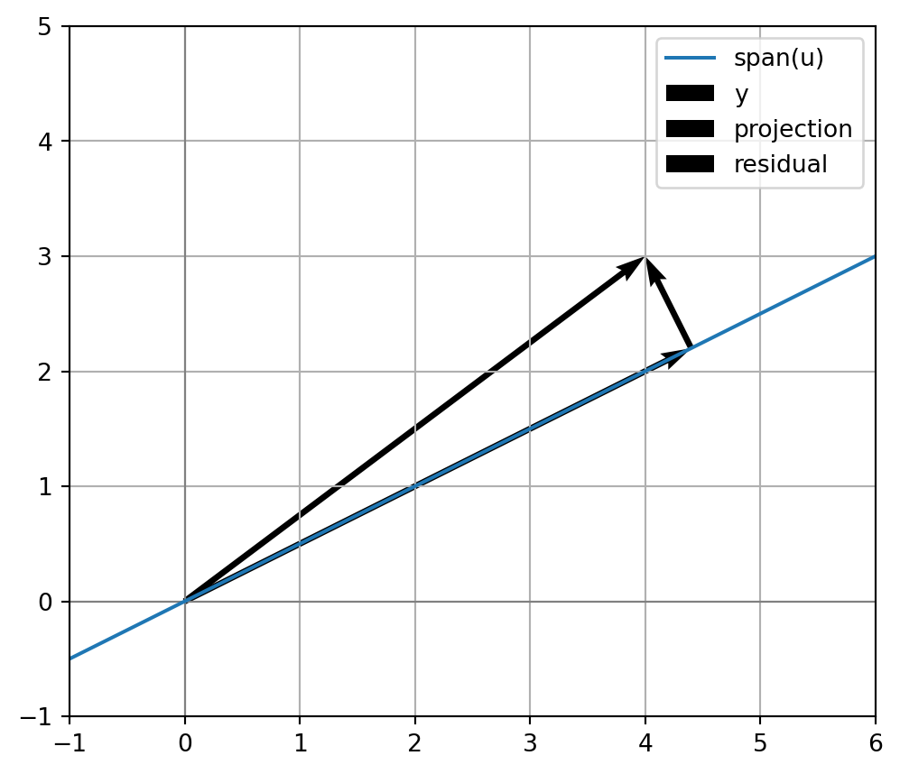
We begin with the simplest case: projecting onto a line.
Let \(u\) be a nonzero vector in \(\mathbb{R}^n\). The line through the origin in the direction \(u\) is
\[
u\cdot r
=2\left(-\frac25\right)+1\left(\frac45\right)=0.
\]
So the error is perpendicular to the line. This perpendicularity is not a coincidence. It is exactly what makes the shadow best.
NoteMeaning
The projection is the part of \(y\) explained by direction \(u\). The residual is the part of \(y\) not explained by direction \(u\).
11.6 11.4 Why Orthogonality Means Best
Why must the residual be perpendicular?
Suppose \(\hat{y}\) is the closest point to \(y\) in a subspace \(S\). If the residual \(r=y-\hat{y}\) had some component along a direction inside \(S\), then we could move slightly inside \(S\) and reduce the error. That would mean \(\hat{y}\) was not the closest point.
Therefore, at the best approximation, there is no leftover direction inside \(S\). The leftover error must point completely outside \(S\).
Mathematically:
\[
r\perp S
\quad \Longleftrightarrow \quad
r\cdot z=0 \text{ for every } z\in S.
\]
This is the orthogonality condition for projection.
ImportantBest approximation theorem
Let \(S\) be a subspace of \(\mathbb{R}^n\). A vector \(\hat{y}\in S\) is the closest vector in \(S\) to \(y\) if and only if
\[
y-\hat{y}\perp S.
\]
11.7 11.5 Projection as Decomposition
Projection breaks a vector into two perpendicular pieces:
\[
y=\hat{y}+r.
\]
Here:
\[
\hat{y}=\operatorname{proj}_S(y)
\]
and
\[
r=y-\hat{y}.
\]
Because \(\hat{y}\) and \(r\) are perpendicular, the Pythagorean theorem gives
\[
\|y\|^2=\|\hat{y}\|^2+\|r\|^2.
\]
This identity is deeply important. It says that the total energy of \(y\) splits into explained energy and unexplained energy.
In data science language:
\(\|\hat{y}\|^2\) is the energy explained by the model space.
\(\|r\|^2\) is the error energy left over.
In statistics, the same idea appears in regression and analysis of variance. In signal processing, it appears when decomposing a signal into useful components and noise.
11.8 11.6 Projection onto an Orthonormal Basis
Projection onto a line is useful, but many approximation spaces have more than one direction.
The projection of \(y\) onto the column space of \(Q\) is
\[
\hat{y}=QQ^Ty.
\]
Thus the projection matrix is
\[
\boxed{P=QQ^T.}
\]
This matrix has two special properties:
\[
P^T=P
\]
and
\[
P^2=P.
\]
The first property says \(P\) is symmetric. The second says projecting twice is the same as projecting once. Once a vector is already on the shadow space, projecting again does not change it.
TipProjection matrices
A matrix \(P\) is an orthogonal projection matrix when it is symmetric and idempotent:
\[
P^T=P,
\qquad
P^2=P.
\]
11.10 11.8 Projection onto a General Column Space
What if the basis vectors are not orthonormal?
Suppose \(A\) is an \(m\times n\) matrix with independent columns. The column space of \(A\) is
We want the closest vector \(\hat{b}\) to \(b\) inside \(\operatorname{Col}(A)\). Since every vector in the column space looks like \(Ax\), we seek
\[
\hat{b}=A\hat{x}
\]
where \(\hat{x}\) minimizes
\[
\|b-Ax\|^2.
\]
The residual is
\[
r=b-A\hat{x}.
\]
For \(A\hat{x}\) to be the best approximation, the residual must be perpendicular to every column of \(A\). That means
\[
A^T(b-A\hat{x})=0.
\]
Rearranging gives the normal equations:
\[
A^TA\hat{x}=A^Tb.
\]
If the columns of \(A\) are independent, \(A^TA\) is invertible, and
\[
\boxed{
\hat{x}=(A^TA)^{-1}A^Tb.
}
\]
The projection itself is
\[
\boxed{
\hat{b}=A(A^TA)^{-1}A^Tb.
}
\]
So the projection matrix onto \(\operatorname{Col}(A)\) is
\[
\boxed{
P=A(A^TA)^{-1}A^T.
}
\]
This formula is the algebraic engine behind least squares.
11.11 11.9 Least Squares: Solving When Exact Solving Is Impossible
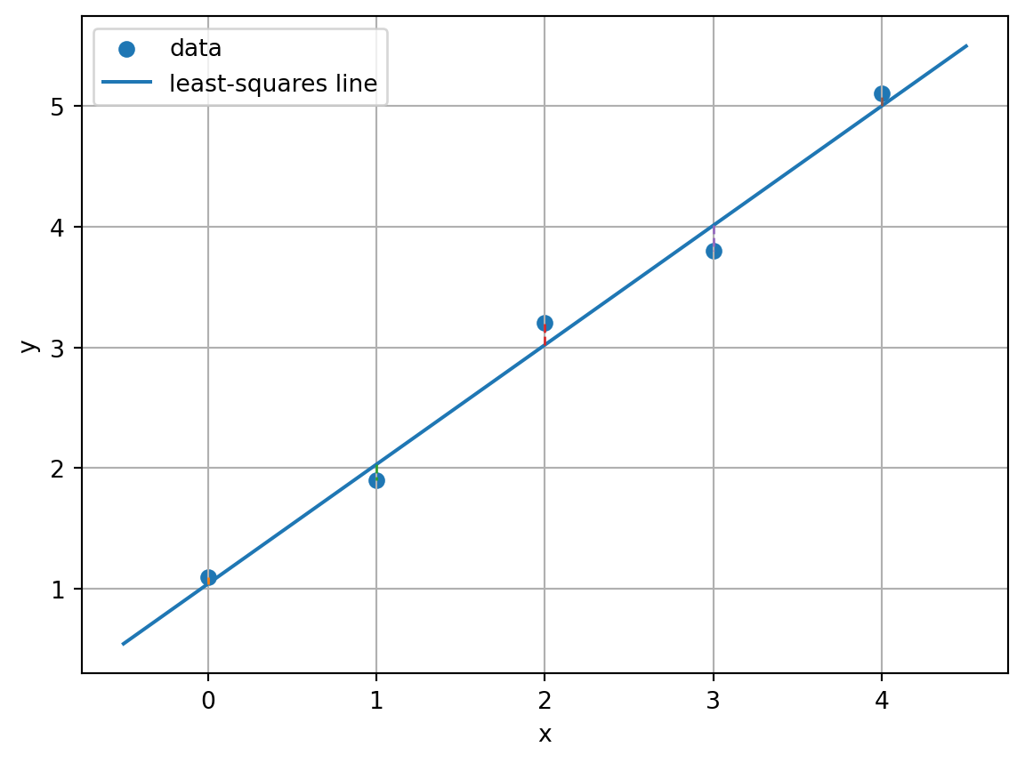
Sometimes \(Ax=b\) has no solution. This often happens when there are more equations than unknowns. In data problems, this is not a failure. It is normal.
For example, suppose many data points roughly follow a line, but not exactly. No single line passes through every point. Instead of solving exactly, we solve approximately:
\[
\min_x \|Ax-b\|^2.
\]
This is called a least-squares problem. The goal is to find the vector \(x\) that makes \(Ax\) as close as possible to \(b\).
The vector \(A\hat{x}\) is the projection of \(b\) onto the column space of \(A\). The residual
\[
r=b-A\hat{x}
\]
is perpendicular to that column space.
This is the geometry behind linear regression.
NoteRegression as projection
In linear regression, the observed response vector \(b\) is projected onto the space spanned by the model features. The fitted values are the projection. The residuals are the part the model cannot explain.
This residual is perpendicular to both columns of \(A\). That means:
\[
A^Tr=0.
\]
The best-fit line is not chosen by magic. It is chosen by orthogonality.
11.13 11.11 Projection and Data Compression
Projection is also a language of compression. Suppose a signal is a long vector \(y\in\mathbb{R}^{1000}\). If we approximate it using only a few basis vectors
\[
q_1,q_2,\ldots,q_k,
\]
then the projection
\[
\hat{y}=\sum_{j=1}^k(q_j\cdot y)q_j
\]
uses only \(k\) numbers:
\[
q_1\cdot y,\ q_2\cdot y,\ldots,\ q_k\cdot y.
\]
The original signal may have 1000 entries. The projected version may use only 10 or 20 coefficients. This is the beginning of Fourier approximation, wavelets, PCA, and image compression.
Projection tells us how to compress while losing as little as possible relative to the chosen approximation space.
11.14 11.12 Projection in Machine Learning
Projection appears throughout machine learning.
11.14.1 Feature models
A model often represents an output vector \(b\) using combinations of feature columns:
\[
b\approx Ax.
\]
Training the model means finding the best combination of features. That is a least-squares projection problem when the loss is squared error.
11.14.2 Embeddings
In text and image models, high-dimensional objects are often projected into lower-dimensional spaces. The goal is to keep important structure while reducing complexity.
11.14.3 Recommendation systems
A user’s preference vector may be approximated using a low-dimensional taste space. The projection is the part explained by the model. The residual is what the model misses.
11.14.4 Neural networks
Each linear layer computes a matrix transformation. Training often tries to find transformations that project data into spaces where patterns become easier to separate.
Projection is not only a formula. It is a way of thinking:
Find the best representation inside the space your model can express.
11.18.1 Misunderstanding 1: Projection keeps everything important
Projection keeps what lies in the chosen subspace. If the subspace is poorly chosen, the projection may lose important information. The quality of approximation depends on the approximation space.
11.18.2 Misunderstanding 2: The residual is always small
The residual is as small as possible among all choices in the subspace, but it may still be large. A best shadow can still be a bad representation if the wall is in the wrong place.
11.18.3 Misunderstanding 3: Least squares solves \(Ax=b\)
Least squares does not necessarily solve \(Ax=b\) exactly. It solves
Projection often lowers dimension, but a projection matrix acts on the original ambient space. For example, a projection matrix in \(\mathbb{R}^3\) can output another vector in \(\mathbb{R}^3\), even though the output lies on a plane.
Why does projecting twice give the same result as projecting once?
What can go wrong if the columns of \(A\) are nearly dependent in a least-squares problem?
Explain why \(A^Tr=0\) means the residual is orthogonal to the model space.
In a regression problem, what does a large residual mean geometrically?
How does projection prepare the way for PCA?
11.21 11.19 AI Companion Activities
Use an AI assistant as a tutor, not as a replacement for your own reasoning.
11.21.1 Activity 1: Explain the picture
Ask:
Explain projection onto a line using only geometry. Do not use formulas until the end.
Then draw your own diagram and label \(y\), \(\hat{y}\), and \(r\).
11.21.2 Activity 2: Check a computation
Ask:
I projected \(y=(3,4)\) onto \(u=(1,2)\). Check my work step by step and explain where the orthogonality condition appears.
11.21.3 Activity 3: Compare formulas
Ask:
Compare \(P=QQ^T\) and \(P=A(A^TA)^{-1}A^T\). When can I use each formula?
11.21.4 Activity 4: Regression as projection
Ask:
Explain linear regression as projection of a response vector onto the column space of a design matrix.
Then write the explanation in your own words.
11.22 11.20 Summary
Projection is one of the central bridges between geometry and computation.
The key ideas are:
Projection finds the closest vector in a chosen subspace.
The residual is perpendicular to the approximation space.
Projection decomposes a vector as \(y=\hat{y}+r\).
Projection onto a line is computed by \(\frac{u\cdot y}{u\cdot u}u\).
Projection onto an orthonormal basis is computed by summing components.
If \(Q\) has orthonormal columns, the projection matrix is \(P=QQ^T\).
If \(A\) has independent columns, the projection matrix onto \(\operatorname{Col}(A)\) is \(P=A(A^TA)^{-1}A^T\).
Least squares is projection when exact solving is impossible.
Projection is the language of best approximation.
The next chapter continues this geometric story. Projection already uses perpendicularity. Now we will study orthogonality as a structure in its own right.
Source Code
---title: "Chapter 11: Projection — The Best Shadow"subtitle: "Best approximation, residuals, least squares, and the geometry of being as close as possible"format: html: toc: true toc-depth: 3 number-sections: true code-fold: true code-tools: true fig-align: centerjupyter: python3---## Opening Story: The Shadow That Loses the LeastImagine a complicated object in three-dimensional space: a person, a building, a cloud, a moving airplane.Now shine a light on it and look at the shadow on a wall.The shadow is simpler than the original object.It has fewer dimensions.It has lost information.Yet it is not random.It is the version of the object that remains after we keep only the part that can be seen from a chosen direction.Projection is the mathematical version of this idea.A projection takes a vector and replaces it by its best shadow on a simpler space: a line, a plane, or a subspace.The word **best** is crucial.Projection is not merely throwing information away.It is throwing information away in the most controlled possible way.Among all vectors in the simpler space, the projection is the one closest to the original vector.This chapter introduces one of the most important principles in applied linear algebra:> When we cannot represent something exactly, we often represent it by the closest thing we can build.That closest thing is a projection.The leftover part is called the **residual**.The magic fact is that the residual is perpendicular to the space of approximation.In the language of this book:> Projection is the best shadow, and orthogonality explains why it is best.This idea becomes the heart of least squares, regression, signal approximation, PCA, image compression, recommendation systems, and many algorithms in machine learning.## Learning GoalsBy the end of this chapter, you should be able to:1. Explain projection as a closest-point problem.2. Compute the projection of a vector onto a line.3. Interpret the projection coefficient as the amount of one direction inside another vector.4. Explain why the residual is orthogonal to the approximation space.5. Use projection to decompose a vector into a visible part and an invisible error part.6. Compute projections onto subspaces with orthonormal bases.7. Understand the matrix formula $P = QQ^T$ for orthogonal projection.8. Understand the least-squares formula $\hat{x}=(A^TA)^{-1}A^Tb$ when the columns of $A$ are independent.9. Use Python to visualize projections, residuals, and least-squares fits.10. Connect projection to data science, regression, signal processing, and machine learning.## 11.1 Projection as a Closest-Point ProblemLet $y$ be a vector in $\mathbb{R}^n$.Let $S$ be a subspace of $\mathbb{R}^n$.The **projection of $y$ onto $S$** is the vector $\hat{y}$ in $S$ that is closest to $y$:$$\hat{y}=\operatorname{proj}_S(y).$$This means that $\hat{y}$ solves the optimization problem$$\hat{y}=\arg\min_{z\in S}\|y-z\|.$$The vector$$r=y-\hat{y}$$is called the **residual** or **error vector**.It measures what remains after the best approximation has been made.The fundamental geometry is:$$y=\hat{y}+r,$$where$$\hat{y}\in S\qquad \text{and} \qquadr\perp S.$$This says:- $\hat{y}$ is the part of $y$ that lives in the subspace $S$.- $r$ is the part of $y$ that cannot be explained by $S$.- The explained part and unexplained part are perpendicular.This is the main picture of the chapter.::: {.callout-tip title="The projection principle"}The best approximation from a subspace is found when the error is perpendicular to every direction inside that subspace.:::## 11.2 Projection onto a LineWe begin with the simplest case: projecting onto a line.Let $u$ be a nonzero vector in $\mathbb{R}^n$.The line through the origin in the direction $u$ is$$L=\operatorname{span}(u)=\{cu:c\in\mathbb{R}\}.$$The projection of $y$ onto $L$ must be some scalar multiple of $u$:$$\hat{y}=cu.$$The best scalar $c$ is chosen so that the residual$$r=y-cu$$is perpendicular to $u$.Therefore$$u\cdot (y-cu)=0.$$Expanding gives$$u\cdot y-c(u\cdot u)=0.$$So$$c=\frac{u\cdot y}{u\cdot u}.$$Therefore the projection formula is$$\boxed{\operatorname{proj}_{\operatorname{span}(u)}(y)=\frac{u\cdot y}{u\cdot u}u.}$$If $u$ is a unit vector, then $u\cdot u=1$, so the formula becomes$$\operatorname{proj}_{\operatorname{span}(u)}(y)=(u\cdot y)u.$$The dot product $u\cdot y$ measures how much $y$ points in the direction of $u$.## 11.3 Worked Example: A Shadow on a DirectionLet$$y=\begin{bmatrix}4\\3\end{bmatrix},\qquadu=\begin{bmatrix}2\\1\end{bmatrix}.$$Then$$u\cdot y=2\cdot 4+1\cdot 3=11$$and$$u\cdot u=2^2+1^2=5.$$Thus$$c=\frac{11}{5}$$and$$\hat{y}=\frac{11}{5}\begin{bmatrix}2\\1\end{bmatrix}=\begin{bmatrix}22/5\\11/5\end{bmatrix}.$$The residual is$$r=y-\hat{y}=\begin{bmatrix}4\\3\end{bmatrix}-\begin{bmatrix}22/5\\11/5\end{bmatrix}=\begin{bmatrix}-2/5\\4/5\end{bmatrix}.$$Check orthogonality:$$u\cdot r=2\left(-\frac25\right)+1\left(\frac45\right)=0.$$So the error is perpendicular to the line.This perpendicularity is not a coincidence.It is exactly what makes the shadow best.::: {.callout-note title="Meaning"}The projection is the part of $y$ explained by direction $u$.The residual is the part of $y$ not explained by direction $u$.:::## 11.4 Why Orthogonality Means BestWhy must the residual be perpendicular?Suppose $\hat{y}$ is the closest point to $y$ in a subspace $S$.If the residual $r=y-\hat{y}$ had some component along a direction inside $S$, then we could move slightly inside $S$ and reduce the error.That would mean $\hat{y}$ was not the closest point.Therefore, at the best approximation, there is no leftover direction inside $S$.The leftover error must point completely outside $S$.Mathematically:$$r\perp S\quad \Longleftrightarrow \quadr\cdot z=0 \text{ for every } z\in S.$$This is the **orthogonality condition for projection**.::: {.callout-important title="Best approximation theorem"}Let $S$ be a subspace of $\mathbb{R}^n$.A vector $\hat{y}\in S$ is the closest vector in $S$ to $y$ if and only if$$y-\hat{y}\perp S.$$:::## 11.5 Projection as DecompositionProjection breaks a vector into two perpendicular pieces:$$y=\hat{y}+r.$$Here:$$\hat{y}=\operatorname{proj}_S(y)$$and$$r=y-\hat{y}.$$Because $\hat{y}$ and $r$ are perpendicular, the Pythagorean theorem gives$$\|y\|^2=\|\hat{y}\|^2+\|r\|^2.$$This identity is deeply important.It says that the total energy of $y$ splits into explained energy and unexplained energy.In data science language:- $\|\hat{y}\|^2$ is the energy explained by the model space.- $\|r\|^2$ is the error energy left over.In statistics, the same idea appears in regression and analysis of variance.In signal processing, it appears when decomposing a signal into useful components and noise.## 11.6 Projection onto an Orthonormal BasisProjection onto a line is useful, but many approximation spaces have more than one direction.Suppose $S$ is spanned by orthonormal vectors$$q_1,q_2,\ldots,q_k.$$Orthonormal means:$$q_i\cdot q_j=0 \text{ if } i\ne j,\qquadq_i\cdot q_i=1.$$Then the projection of $y$ onto $S$ is$$\boxed{\operatorname{proj}_S(y)=(q_1\cdot y)q_1+(q_2\cdot y)q_2+\cdots+(q_k\cdot y)q_k.}$$Each coefficient $q_i\cdot y$ measures how much of $y$ lies in direction $q_i$.This is one reason orthonormal bases are so powerful.They make projection simple.Each direction can be handled independently.## 11.7 The Projection Matrix $P=QQ^T$Put the orthonormal vectors into a matrix:$$Q=\begin{bmatrix}q_1&q_2&\cdots&q_k\end{bmatrix}.$$The columns of $Q$ are orthonormal, so$$Q^TQ=I_k.$$The projection of $y$ onto the column space of $Q$ is$$\hat{y}=QQ^Ty.$$Thus the projection matrix is$$\boxed{P=QQ^T.}$$This matrix has two special properties:$$P^T=P$$and$$P^2=P.$$The first property says $P$ is symmetric.The second says projecting twice is the same as projecting once.Once a vector is already on the shadow space, projecting again does not change it.::: {.callout-tip title="Projection matrices"}A matrix $P$ is an orthogonal projection matrix when it is symmetric and idempotent:$$P^T=P,\qquadP^2=P.$$:::## 11.8 Projection onto a General Column SpaceWhat if the basis vectors are not orthonormal?Suppose $A$ is an $m\times n$ matrix with independent columns.The column space of $A$ is$$\operatorname{Col}(A)=\{Ax:x\in\mathbb{R}^n\}.$$We want the closest vector $\hat{b}$ to $b$ inside $\operatorname{Col}(A)$.Since every vector in the column space looks like $Ax$, we seek$$\hat{b}=A\hat{x}$$where $\hat{x}$ minimizes$$\|b-Ax\|^2.$$The residual is$$r=b-A\hat{x}.$$For $A\hat{x}$ to be the best approximation, the residual must be perpendicular to every column of $A$.That means$$A^T(b-A\hat{x})=0.$$Rearranging gives the **normal equations**:$$A^TA\hat{x}=A^Tb.$$If the columns of $A$ are independent, $A^TA$ is invertible, and$$\boxed{\hat{x}=(A^TA)^{-1}A^Tb.}$$The projection itself is$$\boxed{\hat{b}=A(A^TA)^{-1}A^Tb.}$$So the projection matrix onto $\operatorname{Col}(A)$ is$$\boxed{P=A(A^TA)^{-1}A^T.}$$This formula is the algebraic engine behind least squares.## 11.9 Least Squares: Solving When Exact Solving Is ImpossibleSometimes $Ax=b$ has no solution.This often happens when there are more equations than unknowns.In data problems, this is not a failure.It is normal.For example, suppose many data points roughly follow a line, but not exactly.No single line passes through every point.Instead of solving exactly, we solve approximately:$$\min_x \|Ax-b\|^2.$$This is called a **least-squares problem**.The goal is to find the vector $x$ that makes $Ax$ as close as possible to $b$.The vector $A\hat{x}$ is the projection of $b$ onto the column space of $A$.The residual$$r=b-A\hat{x}$$is perpendicular to that column space.This is the geometry behind linear regression.::: {.callout-note title="Regression as projection"}In linear regression, the observed response vector $b$ is projected onto the space spanned by the model features.The fitted values are the projection.The residuals are the part the model cannot explain.:::## 11.10 Example: Fitting a LineSuppose we observe three data points:$$(0,1),\quad (1,2),\quad (2,2).$$We want to fit a line$$y\approx c+mx.$$The equations would be$$\begin{aligned}c+0m &\approx 1,\\c+1m &\approx 2,\\c+2m &\approx 2.\end{aligned}$$In matrix form:$$A\begin{bmatrix}c\\m\end{bmatrix}\approx b,$$where$$A=\begin{bmatrix}1&0\\1&1\\1&2\end{bmatrix},\qquadb=\begin{bmatrix}1\\2\\2\end{bmatrix}.$$The least-squares solution is$$\hat{x}=(A^TA)^{-1}A^Tb.$$A calculation gives$$\hat{x}=\begin{bmatrix}7/6\\1/2\end{bmatrix}.$$So the best-fit line is$$y\approx \frac76+\frac12 x.$$The fitted values are$$A\hat{x}=\begin{bmatrix}7/6\\5/3\\13/6\end{bmatrix}.$$The residual vector is$$r=b-A\hat{x}=\begin{bmatrix}-1/6\\1/3\\-1/6\end{bmatrix}.$$This residual is perpendicular to both columns of $A$.That means:$$A^Tr=0.$$The best-fit line is not chosen by magic.It is chosen by orthogonality.## 11.11 Projection and Data CompressionProjection is also a language of compression.Suppose a signal is a long vector $y\in\mathbb{R}^{1000}$.If we approximate it using only a few basis vectors$$q_1,q_2,\ldots,q_k,$$then the projection$$\hat{y}=\sum_{j=1}^k(q_j\cdot y)q_j$$uses only $k$ numbers:$$q_1\cdot y,\ q_2\cdot y,\ldots,\ q_k\cdot y.$$The original signal may have 1000 entries.The projected version may use only 10 or 20 coefficients.This is the beginning of Fourier approximation, wavelets, PCA, and image compression.Projection tells us how to compress while losing as little as possible relative to the chosen approximation space.## 11.12 Projection in Machine LearningProjection appears throughout machine learning.### Feature modelsA model often represents an output vector $b$ using combinations of feature columns:$$b\approx Ax.$$Training the model means finding the best combination of features.That is a least-squares projection problem when the loss is squared error.### EmbeddingsIn text and image models, high-dimensional objects are often projected into lower-dimensional spaces.The goal is to keep important structure while reducing complexity.### Recommendation systemsA user's preference vector may be approximated using a low-dimensional taste space.The projection is the part explained by the model.The residual is what the model misses.### Neural networksEach linear layer computes a matrix transformation.Training often tries to find transformations that project data into spaces where patterns become easier to separate.Projection is not only a formula.It is a way of thinking:> Find the best representation inside the space your model can express.## 11.13 Python: Projection onto a Line```{python}import numpy as npimport matplotlib.pyplot as plt# Vector to project and direction vectory = np.array([4.0, 3.0])u = np.array([2.0, 1.0])# Projection onto span(u)proj = (np.dot(u, y) / np.dot(u, u)) * uresid = y - projprint("y =", y)print("u =", u)print("projection =", proj)print("residual =", resid)print("u dot residual =", np.dot(u, resid))# Plotfig, ax = plt.subplots(figsize=(6, 6))ax.axhline(0, color="gray", linewidth=0.8)ax.axvline(0, color="gray", linewidth=0.8)# Draw line span(u)ts = np.linspace(-1, 3, 100)line = np.outer(ts, u)ax.plot(line[:, 0], line[:, 1], label="span(u)")# Vectorsax.quiver(0, 0, y[0], y[1], angles="xy", scale_units="xy", scale=1, label="y")ax.quiver(0, 0, proj[0], proj[1], angles="xy", scale_units="xy", scale=1, label="projection")ax.quiver(proj[0], proj[1], resid[0], resid[1], angles="xy", scale_units="xy", scale=1, label="residual")ax.set_xlim(-1, 6)ax.set_ylim(-1, 5)ax.set_aspect("equal")ax.grid(True)ax.legend()plt.show()```## 11.14 Python: Least-Squares Line Fitting```{python}import numpy as npimport matplotlib.pyplot as plt# Data pointsx_data = np.array([0, 1, 2, 3, 4], dtype=float)y_data = np.array([1.1, 1.9, 3.2, 3.8, 5.1], dtype=float)# Design matrix for y ≈ c + mxA = np.column_stack([np.ones_like(x_data), x_data])b = y_data# Least-squares solutionx_hat = np.linalg.solve(A.T @ A, A.T @ b)c, m = x_hatfitted = A @ x_hatresidual = b - fittedprint("intercept c =", c)print("slope m =", m)print("residual =", residual)print("A.T @ residual =", A.T @ residual)# Plot data and fitxx = np.linspace(-0.5, 4.5, 200)yy = c + m * xxplt.figure(figsize=(7, 5))plt.scatter(x_data, y_data, label="data")plt.plot(xx, yy, label="least-squares line")for xi, yi, fi inzip(x_data, y_data, fitted): plt.plot([xi, xi], [fi, yi], linestyle="--", linewidth=1)plt.grid(True)plt.xlabel("x")plt.ylabel("y")plt.legend()plt.show()```## 11.15 Python: Projection with an Orthonormal Basis```{python}import numpy as np# Build a random subspace in R^5 with dimension 2rng = np.random.default_rng(7)B = rng.normal(size=(5, 2))# QR gives orthonormal columns QQ, R = np.linalg.qr(B)y = rng.normal(size=5)proj = Q @ (Q.T @ y)resid = y - projprint("Q.T @ Q =")print(np.round(Q.T @ Q, 6))print("projection =", np.round(proj, 4))print("residual =", np.round(resid, 4))print("Q.T @ residual =", np.round(Q.T @ resid, 10))print("||y||^2 =", np.dot(y, y))print("||proj||^2 + ||resid||^2 =", np.dot(proj, proj) + np.dot(resid, resid))```## 11.16 Common Misunderstandings### Misunderstanding 1: Projection keeps everything importantProjection keeps what lies in the chosen subspace.If the subspace is poorly chosen, the projection may lose important information.The quality of approximation depends on the approximation space.### Misunderstanding 2: The residual is always smallThe residual is as small as possible among all choices in the subspace, but it may still be large.A best shadow can still be a bad representation if the wall is in the wrong place.### Misunderstanding 3: Least squares solves $Ax=b$Least squares does not necessarily solve $Ax=b$ exactly.It solves$$Ax\approx b$$by making the error as small as possible.### Misunderstanding 4: Projection always lowers dimensionProjection often lowers dimension, but a projection matrix acts on the original ambient space.For example, a projection matrix in $\mathbb{R}^3$ can output another vector in $\mathbb{R}^3$, even though the output lies on a plane.## 11.17 Practice Problems### Problem 1: Projection onto a lineLet$$y=\begin{bmatrix}3\\4\end{bmatrix},\qquadu=\begin{bmatrix}1\\2\end{bmatrix}.$$Find $\operatorname{proj}_{\operatorname{span}(u)}(y)$ and the residual $r$.Verify that $r\perp u$.::: {.callout-caution collapse="true" title="Solution"}We compute$$u\cdot y=1\cdot 3+2\cdot 4=11$$and$$u\cdot u=1^2+2^2=5.$$So$$\operatorname{proj}_{\operatorname{span}(u)}(y)=\frac{11}{5}\begin{bmatrix}1\\2\end{bmatrix}=\begin{bmatrix}11/5\\22/5\end{bmatrix}.$$The residual is$$r=\begin{bmatrix}3\\4\end{bmatrix}-\begin{bmatrix}11/5\\22/5\end{bmatrix}=\begin{bmatrix}4/5\\-2/5\end{bmatrix}.$$Check:$$u\cdot r=1\cdot \frac45+2\cdot\left(-\frac25\right)=0.$$:::### Problem 2: Projection with a unit vectorLet $q=(1/\sqrt{2},1/\sqrt{2})^T$ and $y=(5,1)^T$.Compute $\operatorname{proj}_{\operatorname{span}(q)}(y)$.::: {.callout-caution collapse="true" title="Solution"}Since $q$ is a unit vector,$$\operatorname{proj}_{\operatorname{span}(q)}(y)=(q\cdot y)q.$$Now$$q\cdot y=\frac{5}{\sqrt2}+\frac{1}{\sqrt2}=\frac{6}{\sqrt2}=3\sqrt2.$$Thus$$(3\sqrt2)q=(3\sqrt2)\begin{bmatrix}1/\sqrt2\\1/\sqrt2\end{bmatrix}=\begin{bmatrix}3\\3\end{bmatrix}.$$:::### Problem 3: Projection matrixLet$$q=\frac{1}{3}\begin{bmatrix}2\\1\\2\end{bmatrix}.$$Find the projection matrix onto $\operatorname{span}(q)$.::: {.callout-caution collapse="true" title="Solution"}Since $q$ is a unit vector, the projection matrix is$$P=qq^T.$$Therefore$$P=\frac{1}{9}\begin{bmatrix}2\\1\\2\end{bmatrix}\begin{bmatrix}2&1&2\end{bmatrix}=\frac{1}{9}\begin{bmatrix}4&2&4\\2&1&2\\4&2&4\end{bmatrix}.$$:::### Problem 4: Least squaresLet$$A=\begin{bmatrix}1&0\\1&1\\1&2\end{bmatrix},\qquadb=\begin{bmatrix}1\\2\\4\end{bmatrix}.$$Find the least-squares solution $\hat{x}$.::: {.callout-caution collapse="true" title="Solution"}The normal equations are$$A^TA\hat{x}=A^Tb.$$Compute$$A^TA=\begin{bmatrix}3&3\\3&5\end{bmatrix},\qquadA^Tb=\begin{bmatrix}7\\10\end{bmatrix}.$$Solving gives$$\hat{x}=\begin{bmatrix}2/3\\3/2\end{bmatrix}.$$So the least-squares line is$$y\approx \frac23+\frac32x.$$:::## 11.18 Challenge Questions1. Why does projecting twice give the same result as projecting once?2. What can go wrong if the columns of $A$ are nearly dependent in a least-squares problem?3. Explain why $A^Tr=0$ means the residual is orthogonal to the model space.4. In a regression problem, what does a large residual mean geometrically?5. How does projection prepare the way for PCA?## 11.19 AI Companion ActivitiesUse an AI assistant as a tutor, not as a replacement for your own reasoning.### Activity 1: Explain the pictureAsk:> Explain projection onto a line using only geometry. Do not use formulas until the end.Then draw your own diagram and label $y$, $\hat{y}$, and $r$.### Activity 2: Check a computationAsk:> I projected $y=(3,4)$ onto $u=(1,2)$. Check my work step by step and explain where the orthogonality condition appears.### Activity 3: Compare formulasAsk:> Compare $P=QQ^T$ and $P=A(A^TA)^{-1}A^T$. When can I use each formula?### Activity 4: Regression as projectionAsk:> Explain linear regression as projection of a response vector onto the column space of a design matrix.Then write the explanation in your own words.## 11.20 SummaryProjection is one of the central bridges between geometry and computation.The key ideas are:- Projection finds the closest vector in a chosen subspace.- The residual is perpendicular to the approximation space.- Projection decomposes a vector as $y=\hat{y}+r$.- Projection onto a line is computed by $\frac{u\cdot y}{u\cdot u}u$.- Projection onto an orthonormal basis is computed by summing components.- If $Q$ has orthonormal columns, the projection matrix is $P=QQ^T$.- If $A$ has independent columns, the projection matrix onto $\operatorname{Col}(A)$ is $P=A(A^TA)^{-1}A^T$.- Least squares is projection when exact solving is impossible.- Projection is the language of best approximation.The next chapter continues this geometric story.Projection already uses perpendicularity.Now we will study orthogonality as a structure in its own right.