---
title: "Chapter 9: Length and Distance"
subtitle: "Measuring size, difference, error, and similarity"
format:
html:
toc: true
toc-depth: 3
number-sections: true
code-fold: true
code-tools: true
jupyter: python3
---
## Opening Story: When Numbers Need a Ruler
In the previous chapters, we learned that a dataset can be viewed as a cloud of points and that a matrix can move, mix, stretch, or collapse those points. But one question has been waiting quietly in the background:
**How do we measure how much something changed?**
Suppose we describe three apartments by four features:
$$
\text{apartment}=
\begin{bmatrix}
\text{rent}\\
\text{square feet}\\
\text{distance to campus}\\
\text{number of bedrooms}
\end{bmatrix}.
$$
One apartment is
$$
x=\begin{bmatrix}2400\\800\\1.2\\2\end{bmatrix},
$$
and another is
$$
y=\begin{bmatrix}2600\\760\\0.8\\2\end{bmatrix}.
$$
Are these apartments similar?
The answer depends on what we mean by **similar**. The rent changed by $200$. The size changed by $40$. The distance changed by $0.4$. The number of bedrooms did not change. These are all numbers, but they do not have the same meaning, the same units, or the same scale.
Linear algebra gives us a first ruler for vector space:
$$
\text{difference}=x-y,
\qquad
\text{distance}=\|x-y\|.
$$
This chapter is about that ruler. We will use it to measure size, difference, error, noise, similarity, and prediction quality.
::: {.callout-important}
## Central Message
Length and distance turn vectors into measurable objects.
Once data points live in a vector space, geometry becomes a way to compare, search, classify, cluster, and learn.
:::
## Learning Goals
By the end of this chapter, you should be able to:
1. Interpret the length of a vector as magnitude, energy, or size.
2. Compute Euclidean norms in $\mathbb{R}^n$.
3. Interpret distance between two vectors as the length of their difference.
4. Explain why feature scaling changes distance-based conclusions.
5. Compare Euclidean distance, Manhattan distance, and maximum distance.
6. Use distance to describe prediction error and residuals.
7. Understand nearest-neighbor thinking in data science.
8. Recognize what changes in high-dimensional spaces.
9. Use Python to compute, visualize, and diagnose distances.
## 9.1 The Length of a Vector
A vector can mean many things: a movement, a data record, an image, a signal, or a prediction error.
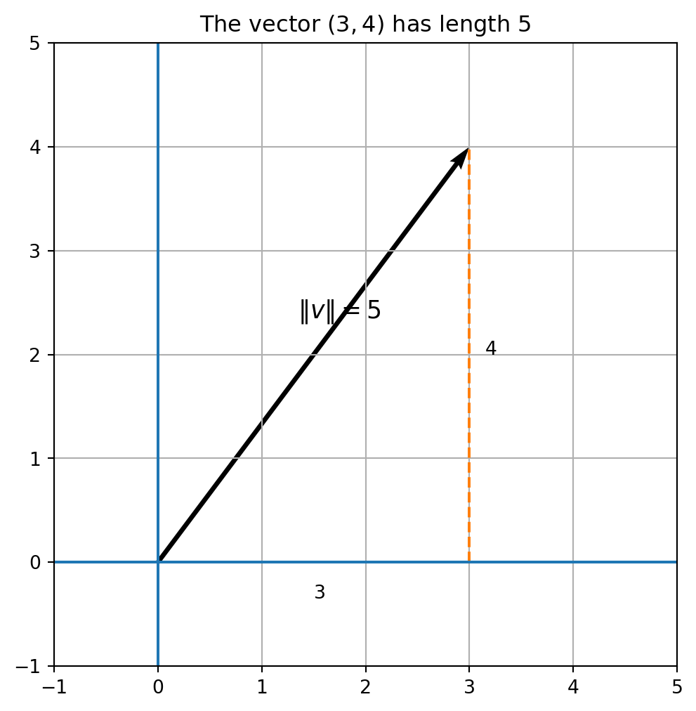
When a vector represents movement, length means how far we moved.
For example,
$$
v=\begin{bmatrix}3\\4\end{bmatrix}
$$
means move $3$ units horizontally and $4$ units vertically. By the Pythagorean theorem,
$$
\|v\|=\sqrt{3^2+4^2}=5.
$$
The notation $\|v\|$ is read as "the norm of $v$" or "the length of $v$."
::: {.callout-note}
## A First Interpretation
For a movement vector, $\|v\|$ is distance traveled.
For a data vector, $\|v\|$ is a measure of total magnitude.
For an error vector, $\|v\|$ is a measure of total error.
:::
```{python}
import numpy as np
import matplotlib.pyplot as plt

v = np.array([3, 4])

plt.figure(figsize=(6, 6))
plt.quiver(0, 0, v[0], v[1], angles="xy", scale_units="xy", scale=1)
plt.plot([0, 3], [0, 0], linestyle="--")
plt.plot([3, 3], [0, 4], linestyle="--")
plt.text(1.5, -0.35, "3")
plt.text(3.15, 2, "4")
plt.text(1.35, 2.35, "$\\|v\\|=5$", fontsize=13)
plt.axhline(0)
plt.axvline(0)
plt.xlim(-1, 5)
plt.ylim(-1, 5)
plt.gca().set_aspect("equal", adjustable="box")
plt.grid(True)
plt.title("The vector $(3,4)$ has length $5$")
plt.show()
```
## 9.2 Euclidean Norm in $\mathbb{R}^n$
The same idea extends to any dimension.
If
$$
v=\begin{bmatrix}v_1\\v_2\\\vdots\\v_n\end{bmatrix}\in \mathbb{R}^n,
$$
then the Euclidean norm is
$$
\|v\|_2=\sqrt{v_1^2+v_2^2+\cdots+v_n^2}.
$$
We often write $\|v\|$ when the Euclidean norm is understood.
::: {.callout-important}
## Definition: Euclidean Norm
For $v\in\mathbb{R}^n$,
$$
\|v\|_2=\sqrt{\sum_{i=1}^n v_i^2}.
$$
:::
### Example: A Five-Dimensional Vector
Let
$$
v=\begin{bmatrix}2\\-1\\3\\0\\4\end{bmatrix}.
$$
Then
$$
\|v\|_2=\sqrt{2^2+(-1)^2+3^2+0^2+4^2}=\sqrt{30}.
$$
```{python}
v = np.array([2, -1, 3, 0, 4])
np.linalg.norm(v)
```
The formula is simple, but the interpretation is powerful. We are measuring the size of an object that may not be drawable.
## 9.3 Distance Between Two Vectors
Distance between two points is the length of the vector connecting them.
If $x,y\in\mathbb{R}^n$, then
$$
d(x,y)=\|x-y\|_2.
$$
The difference vector $x-y$ tells us **how to move from $y$ to $x$**. Its length tells us **how far apart they are**.
::: {.callout-important}
## Definition: Euclidean Distance
For $x,y\in\mathbb{R}^n$,
$$
d(x,y)=\|x-y\|_2
=\sqrt{(x_1-y_1)^2+\cdots+(x_n-y_n)^2}.
$$
:::
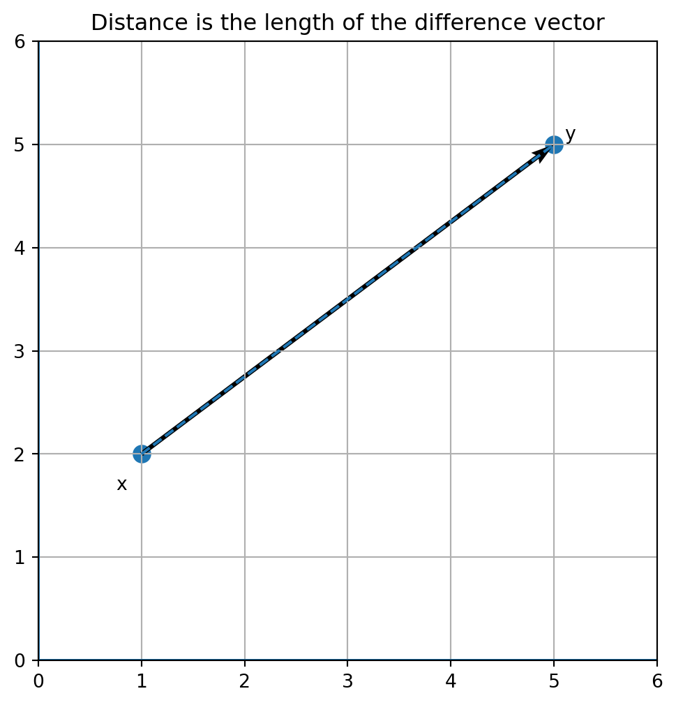
### Example: Distance Between Two Points
Let
$$
x=\begin{bmatrix}1\\2\end{bmatrix},
\qquad
y=\begin{bmatrix}5\\5\end{bmatrix}.
$$
Then
$$
y-x=\begin{bmatrix}4\\3\end{bmatrix},
$$
so
$$
d(x,y)=\sqrt{4^2+3^2}=5.
$$
```{python}
x = np.array([1, 2])
y = np.array([5, 5])

print("difference y - x =", y - x)
print("distance =", np.linalg.norm(y - x))
```
```{python}
plt.figure(figsize=(6, 6))
plt.scatter([x[0], y[0]], [x[1], y[1]], s=80)
plt.text(x[0]-0.25, x[1]-0.35, "x")
plt.text(y[0]+0.1, y[1]+0.05, "y")
plt.quiver(x[0], x[1], y[0]-x[0], y[1]-x[1], angles="xy", scale_units="xy", scale=1)
plt.plot([x[0], y[0]], [x[1], y[1]], linestyle="--")
plt.axhline(0)
plt.axvline(0)
plt.xlim(0, 6)
plt.ylim(0, 6)
plt.grid(True)
plt.gca().set_aspect("equal", adjustable="box")
plt.title("Distance is the length of the difference vector")
plt.show()
```
## 9.4 Distance as Error
One of the most important uses of distance is to measure error.
Suppose a model predicts
$$
\hat y=\begin{bmatrix}3.1\\4.8\\6.2\\7.9\end{bmatrix},
$$
but the true values are
$$
y=\begin{bmatrix}3\\5\\6\\8\end{bmatrix}.
$$
The error vector is
$$
e=y-\hat y.
$$
The norm $\|e\|$ measures total error.
```{python}
y_true = np.array([3, 5, 6, 8])
y_pred = np.array([3.1, 4.8, 6.2, 7.9])
e = y_true - y_pred

print("error vector:", e)
print("total Euclidean error:", np.linalg.norm(e))
print("root mean squared error:", np.sqrt(np.mean(e**2)))
```
::: {.callout-note}
## Error as Geometry
Prediction error is not only a list of mistakes.
It is a vector.
The size of that vector tells us how far the prediction is from the truth.
:::
### Sum of Squared Errors
The square of the Euclidean norm is especially important:
$$
\|e\|_2^2=e_1^2+e_2^2+\cdots+e_n^2.
$$
This is the **sum of squared errors**.
Least squares, regression, PCA, and many machine learning methods are built around minimizing squared distance.
## 9.5 Why Squaring Matters
Why do we square errors?
There are several reasons.
First, positive and negative errors should not cancel. If a model is too high by $10$ and too low by $10$, the total signed error is $0$, but the model still made mistakes.
Second, squaring gives larger mistakes more weight.
Third, squared length has beautiful algebraic properties that connect distance to dot products and projections.
For example, if
$$
e=\begin{bmatrix}3\\4\end{bmatrix},
$$
then
$$
\|e\|_2^2=3^2+4^2=25.
$$
The squared length is often easier to optimize than the length itself.
## 9.6 Unit Vectors and Normalization
A unit vector is a vector with length $1$.
If $v\neq 0$, then
$$
u=\frac{v}{\|v\|}
$$
has length $1$.
This operation is called **normalization**.
::: {.callout-important}
## Definition: Unit Vector
A vector $u$ is a unit vector if
$$
\|u\|=1.
$$
For $v\neq 0$, the vector
$$
\frac{v}{\|v\|}
$$
points in the same direction as $v$ but has length $1$.
:::
```{python}
v = np.array([6, 8])
u = v / np.linalg.norm(v)

print("v =", v)
print("length of v =", np.linalg.norm(v))
print("u =", u)
print("length of u =", np.linalg.norm(u))
```
Normalization separates **direction** from **magnitude**.
This is important in data science. Sometimes we care about the scale of a vector. Sometimes we care only about its direction.
## 9.7 Feature Scaling: The Hidden Trap
Now return to the apartment example.
$$
x=\begin{bmatrix}2400\\800\\1.2\\2\end{bmatrix},
\qquad
y=\begin{bmatrix}2600\\760\\0.8\\2\end{bmatrix}.
$$
The raw difference is
$$
x-y=\begin{bmatrix}-200\\40\\0.4\\0\end{bmatrix}.
$$
The rent coordinate dominates the distance because it is measured in dollars. This does not necessarily mean rent is more important. It may only mean that rent uses larger units.
```{python}
x = np.array([2400, 800, 1.2, 2])
y = np.array([2600, 760, 0.8, 2])

print("raw difference:", x - y)
print("raw distance:", np.linalg.norm(x - y))
```
If we change rent from dollars to thousands of dollars, the distance changes dramatically.
```{python}
x_scaled_units = np.array([2.4, 800, 1.2, 2])
y_scaled_units = np.array([2.6, 760, 0.8, 2])

print("distance after changing rent units:", np.linalg.norm(x_scaled_units - y_scaled_units))
```
::: {.callout-warning}
## Warning: Distance Depends on Units
Distance is not automatically objective.
If features have different units or scales, raw Euclidean distance can be misleading.
Before using distance, ask: **What does one unit in each coordinate mean?**
:::
## 9.8 Standardization
A common solution is to standardize each feature.
For a feature column $x_1,x_2,\ldots,x_m$, we replace each value by
$$
z_i=\frac{x_i-\mu}{\sigma},
$$
where $\mu$ is the mean and $\sigma$ is the standard deviation of that feature.
After standardization, each feature is measured in standard deviation units.
```{python}
X = np.array([
    [2400, 800, 1.2, 2],
    [2600, 760, 0.8, 2],
    [1800, 600, 3.5, 1],
    [3200, 1100, 0.5, 3],
    [2100, 700, 2.2, 2]
], dtype=float)

mu = X.mean(axis=0)
sigma = X.std(axis=0, ddof=0)
Z = (X - mu) / sigma

print("feature means:", mu)
print("feature standard deviations:", sigma)
print("standardized data:\n", np.round(Z, 2))
```
```{python}
from itertools import combinations

def pairwise_distances(A):
    D = np.zeros((len(A), len(A)))
    for i in range(len(A)):
        for j in range(len(A)):
            D[i, j] = np.linalg.norm(A[i] - A[j])
    return D

print("raw distance matrix:\n", np.round(pairwise_distances(X), 1))
print("standardized distance matrix:\n", np.round(pairwise_distances(Z), 2))
```
Standardization does not solve every problem, but it makes distance more meaningful when features have very different scales.
## 9.9 Other Ways to Measure Distance
Euclidean distance is not the only distance.
Different problems need different rulers.
### Manhattan Distance
The Manhattan distance between $x,y\in\mathbb{R}^n$ is
$$
\|x-y\|_1=|x_1-y_1|+\cdots+|x_n-y_n|.
$$
It measures distance as if we must move along coordinate directions, like walking on city blocks.
### Maximum Distance
The maximum distance is
$$
\|x-y\|_\infty=\max_i |x_i-y_i|.
$$
It measures the largest coordinate difference.
### Euclidean Distance
The Euclidean distance is
$$
\|x-y\|_2=\sqrt{(x_1-y_1)^2+\cdots+(x_n-y_n)^2}.
$$
```{python}
x = np.array([1, 2, 5])
y = np.array([4, 6, 1])
diff = x - y

print("L1 distance:", np.sum(np.abs(diff)))
print("L2 distance:", np.linalg.norm(diff))
print("L-infinity distance:", np.max(np.abs(diff)))
```
::: {.callout-note}
## Choosing a Distance
A distance is a modeling choice.
Euclidean distance says that all coordinate errors combine like perpendicular directions.
Manhattan distance says total coordinate-wise change matters.
Maximum distance says the worst coordinate difference matters most.
:::
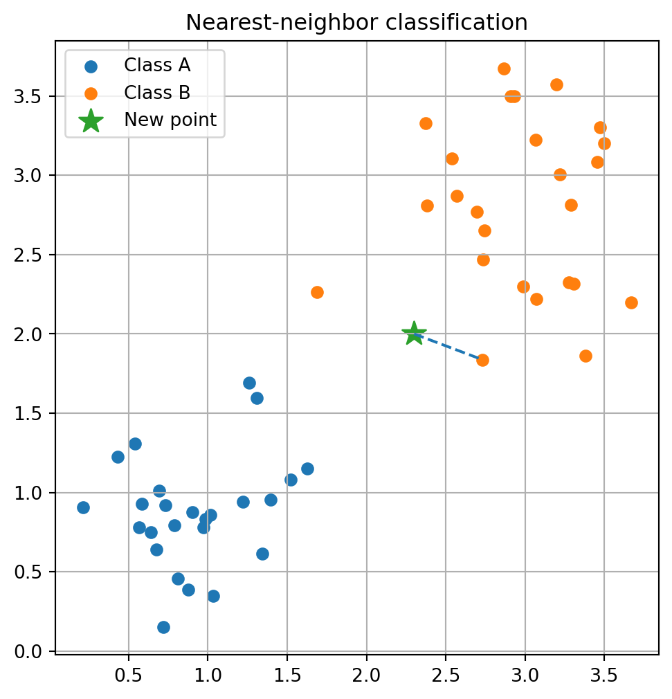
## 9.10 Nearest Neighbors
A simple but powerful idea in data science is this:
> To understand a new point, look at nearby old points.
This is the intuition behind nearest-neighbor methods.
Suppose we have points labeled by class. To classify a new point, we can find the closest labeled point and copy its label.
```{python}
np.random.seed(3)
A = np.random.normal(loc=[1, 1], scale=0.35, size=(25, 2))
B = np.random.normal(loc=[3, 2.7], scale=0.45, size=(25, 2))
new_point = np.array([2.3, 2.0])
X_data = np.vstack([A, B])
labels = np.array([0]*len(A) + [1]*len(B))

distances = np.linalg.norm(X_data - new_point, axis=1)
nearest = np.argmin(distances)

plt.figure(figsize=(7, 6))
plt.scatter(A[:, 0], A[:, 1], label="Class A")
plt.scatter(B[:, 0], B[:, 1], label="Class B")
plt.scatter(new_point[0], new_point[1], marker="*", s=180, label="New point")
plt.plot([new_point[0], X_data[nearest,0]], [new_point[1], X_data[nearest,1]], linestyle="--")
plt.legend()
plt.grid(True)
plt.gca().set_aspect("equal", adjustable="box")
plt.title("Nearest-neighbor classification")
plt.show()

print("nearest label:", "A" if labels[nearest] == 0 else "B")
print("nearest distance:", distances[nearest])
```
Nearest-neighbor methods are intuitive, but they are extremely sensitive to scaling and to the choice of distance.
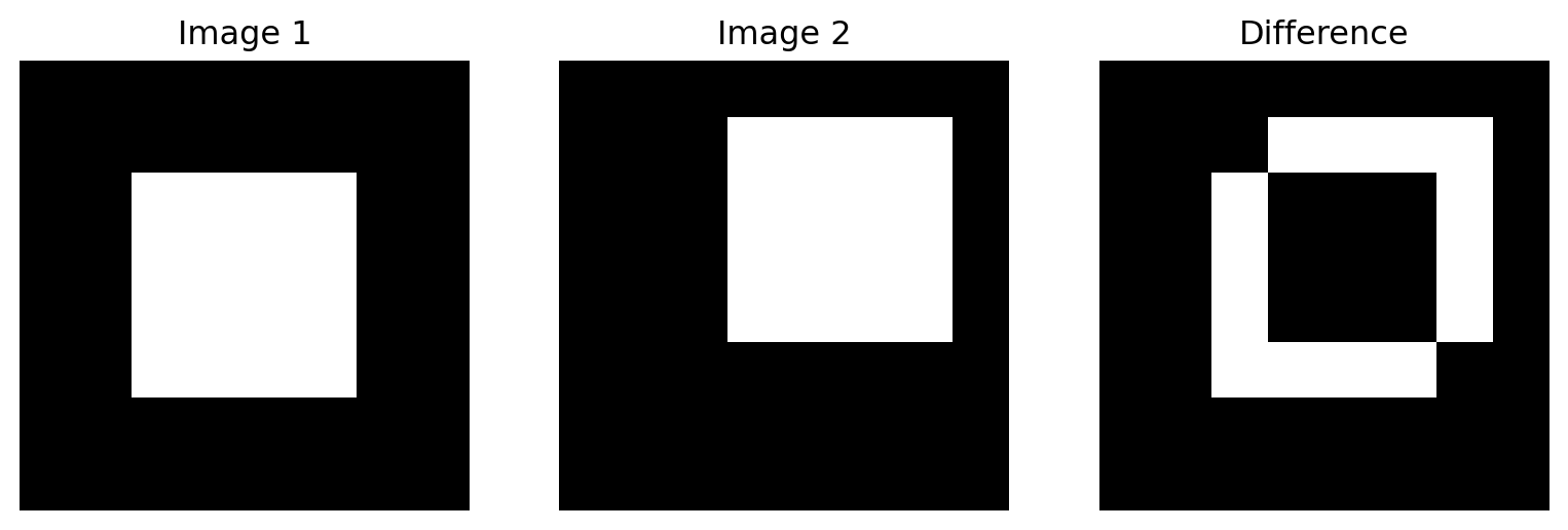
## 9.11 Distance Between Images
An image can be treated as a vector.
A grayscale $8\times 8$ image has $64$ pixel values. If we flatten the image, it becomes a vector in $\mathbb{R}^{64}$.
Then distance between images becomes distance between vectors.
```{python}
img1 = np.zeros((8, 8))
img2 = np.zeros((8, 8))

img1[2:6, 2:6] = 1
img2[1:5, 3:7] = 1

v1 = img1.reshape(-1)
v2 = img2.reshape(-1)

print("image vector dimension:", v1.shape[0])
print("distance between images:", np.linalg.norm(v1 - v2))

fig, axes = plt.subplots(1, 3, figsize=(10, 3))
axes[0].imshow(img1, cmap="gray", vmin=0, vmax=1)
axes[0].set_title("Image 1")
axes[1].imshow(img2, cmap="gray", vmin=0, vmax=1)
axes[1].set_title("Image 2")
axes[2].imshow(np.abs(img1-img2), cmap="gray", vmin=0, vmax=1)
axes[2].set_title("Difference")
for ax in axes:
    ax.axis("off")
plt.show()
```
This idea is important, but it also has a limitation. Two images can have large pixel distance even if they look similar to humans. Later chapters will show how better feature spaces can make distance more meaningful.
## 9.12 High-Dimensional Distance
High-dimensional spaces behave differently from the plane.
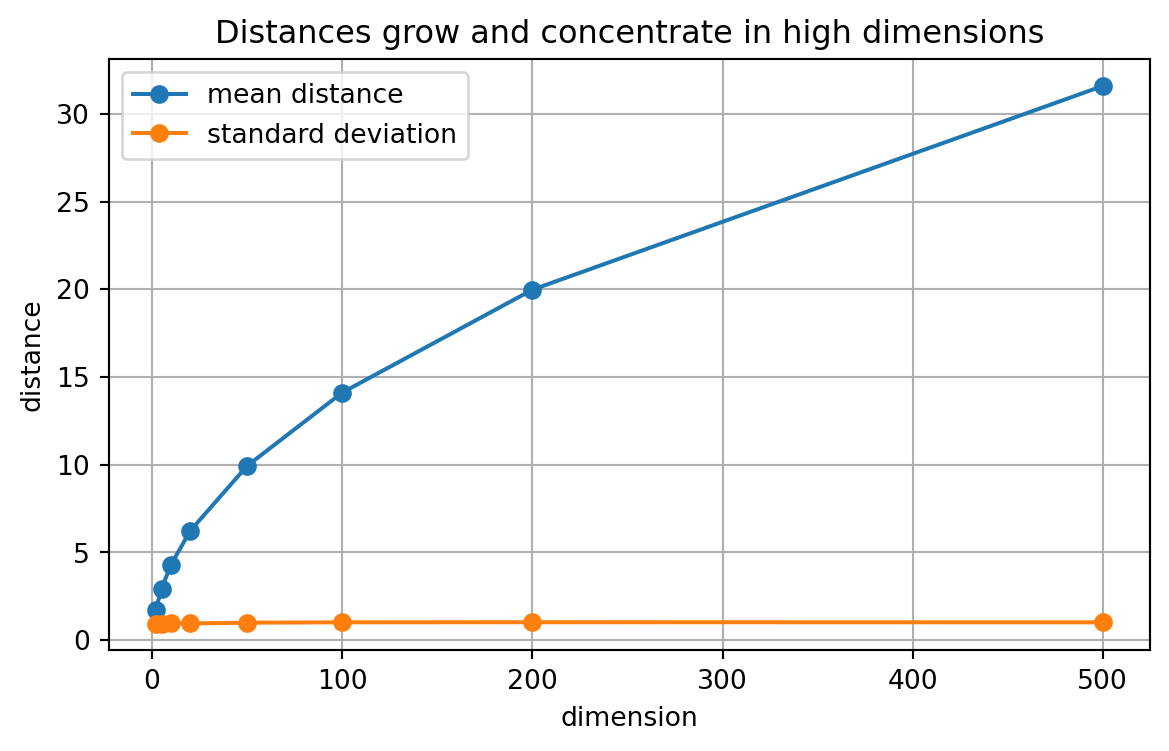
One surprising phenomenon is that random points in high dimensions often become far from one another, and their distances can concentrate.
```{python}
np.random.seed(0)
dimensions = [2, 5, 10, 20, 50, 100, 200, 500]
mean_distances = []
std_distances = []

for d in dimensions:
    X = np.random.normal(size=(500, d))
    Y = np.random.normal(size=(500, d))
    dist = np.linalg.norm(X - Y, axis=1)
    mean_distances.append(dist.mean())
    std_distances.append(dist.std())

plt.figure(figsize=(7, 4))
plt.plot(dimensions, mean_distances, marker="o", label="mean distance")
plt.plot(dimensions, std_distances, marker="o", label="standard deviation")
plt.xlabel("dimension")
plt.ylabel("distance")
plt.title("Distances grow and concentrate in high dimensions")
plt.grid(True)
plt.legend()
plt.show()
```
The mean distance grows roughly like $\sqrt{d}$. The relative variation often becomes smaller.
This matters for machine learning. In high-dimensional spaces, "near" and "far" may not behave the way our two-dimensional intuition suggests.
::: {.callout-warning}
## High-Dimensional Warning
Distance-based intuition from the plane can fail in high dimensions.
In high-dimensional data, distances may become less contrasted, noise can dominate, and feature design becomes crucial.
:::
## 9.13 Distances After a Matrix Transformation
If a matrix $A$ transforms vectors, then distances may change.
For two points $x$ and $y$,
$$
\text{original distance}=\|x-y\|,
$$
while after applying $A$,
$$
\text{new distance}=\|Ax-Ay\|=\|A(x-y)\|.
$$
A rotation preserves distances. A stretch changes distances. A collapse may turn nonzero distance into zero.
```{python}
theta = np.pi / 4
R = np.array([[np.cos(theta), -np.sin(theta)],
              [np.sin(theta),  np.cos(theta)]])
S = np.array([[2, 0],
              [0, 0.5]])
C = np.array([[1, 0],
              [0, 0]])

x = np.array([1, 1])
y = np.array([3, 2])

for name, A in [("rotation", R), ("stretch", S), ("collapse", C)]:
    print(name)
    print("original distance:", np.linalg.norm(x-y))
    print("transformed distance:", np.linalg.norm(A@x - A@y))
    print()
```
This connects distance to everything we learned about matrix machines.
## 9.14 Worked Examples
### Worked Example 1: Compute a Norm
Let
$$
v=\begin{bmatrix}-2\\6\\3\end{bmatrix}.
$$
Then
$$
\|v\|_2=\sqrt{(-2)^2+6^2+3^2}=\sqrt{49}=7.
$$
### Worked Example 2: Compare Two Data Points
Let
$$
x=\begin{bmatrix}2\\5\\1\end{bmatrix},
\qquad
y=\begin{bmatrix}-1\\1\\3\end{bmatrix}.
$$
Then
$$
x-y=\begin{bmatrix}3\\4\\-2\end{bmatrix}
$$
and
$$
d(x,y)=\sqrt{3^2+4^2+(-2)^2}=\sqrt{29}.
$$
### Worked Example 3: Error Vector
Suppose
$$
y=\begin{bmatrix}10\\12\\9\\15\end{bmatrix},
\qquad
\hat y=\begin{bmatrix}11\\10\\10\\14\end{bmatrix}.
$$
Then
$$
e=y-\hat y=\begin{bmatrix}-1\\2\\-1\\1\end{bmatrix}.
$$
The total squared error is
$$
\|e\|^2=1+4+1+1=7.
$$
The root mean squared error is
$$
\sqrt{\frac{7}{4}}.
$$
## 9.15 Practice Problems
### Problem 1
Compute the Euclidean norm of
$$
v=\begin{bmatrix}1\\-2\\2\\4\end{bmatrix}.
$$
::: {.callout-tip collapse="true"}
## Solution
$$
\|v\|=\sqrt{1^2+(-2)^2+2^2+4^2}=\sqrt{25}=5.
$$
:::
### Problem 2
Compute the Euclidean distance between
$$
x=\begin{bmatrix}3\\0\\-1\end{bmatrix},
\qquad
y=\begin{bmatrix}1\\4\\2\end{bmatrix}.
$$
::: {.callout-tip collapse="true"}
## Solution
$$
x-y=\begin{bmatrix}2\\-4\\-3\end{bmatrix}.
$$
Therefore
$$
d(x,y)=\sqrt{2^2+(-4)^2+(-3)^2}=\sqrt{29}.
$$
:::
### Problem 3
Let
$$
v=\begin{bmatrix}5\\12\end{bmatrix}.
$$
Find a unit vector in the same direction as $v$.
::: {.callout-tip collapse="true"}
## Solution
$$
\|v\|=\sqrt{5^2+12^2}=13.
$$
So
$$
u=\frac{1}{13}\begin{bmatrix}5\\12\end{bmatrix}
=\begin{bmatrix}5/13\\12/13\end{bmatrix}.
$$
:::
### Problem 4
A model predicts
$$
\hat y=\begin{bmatrix}2\\4\\5\end{bmatrix},
$$
while the true output is
$$
y=\begin{bmatrix}3\\1\\7\end{bmatrix}.
$$
Compute the error vector, squared error, and RMSE.
::: {.callout-tip collapse="true"}
## Solution
$$
e=y-\hat y=\begin{bmatrix}1\\-3\\2\end{bmatrix}.
$$
The squared error is
$$
\|e\|^2=1^2+(-3)^2+2^2=14.
$$
The RMSE is
$$
\sqrt{\frac{14}{3}}.
$$
:::
### Problem 5
Explain why raw Euclidean distance may be misleading for a dataset with height in meters and income in dollars.
::: {.callout-tip collapse="true"}
## Solution
Income values are usually much larger numerically than height values. Therefore, raw Euclidean distance may be dominated by income. This may reflect units rather than true importance. Scaling or standardization is often needed.
:::
## 9.16 Challenge Questions
1. Can two vectors have the same length but point in very different directions?
2. Can two points be close in Euclidean distance but very different in one important coordinate?
3. Give an example where Manhattan distance is more natural than Euclidean distance.
4. Why might pixel distance fail to match human visual similarity?
5. What does it mean for a matrix transformation to preserve distance?
## 9.17 Python Exploration: Distance Matrix
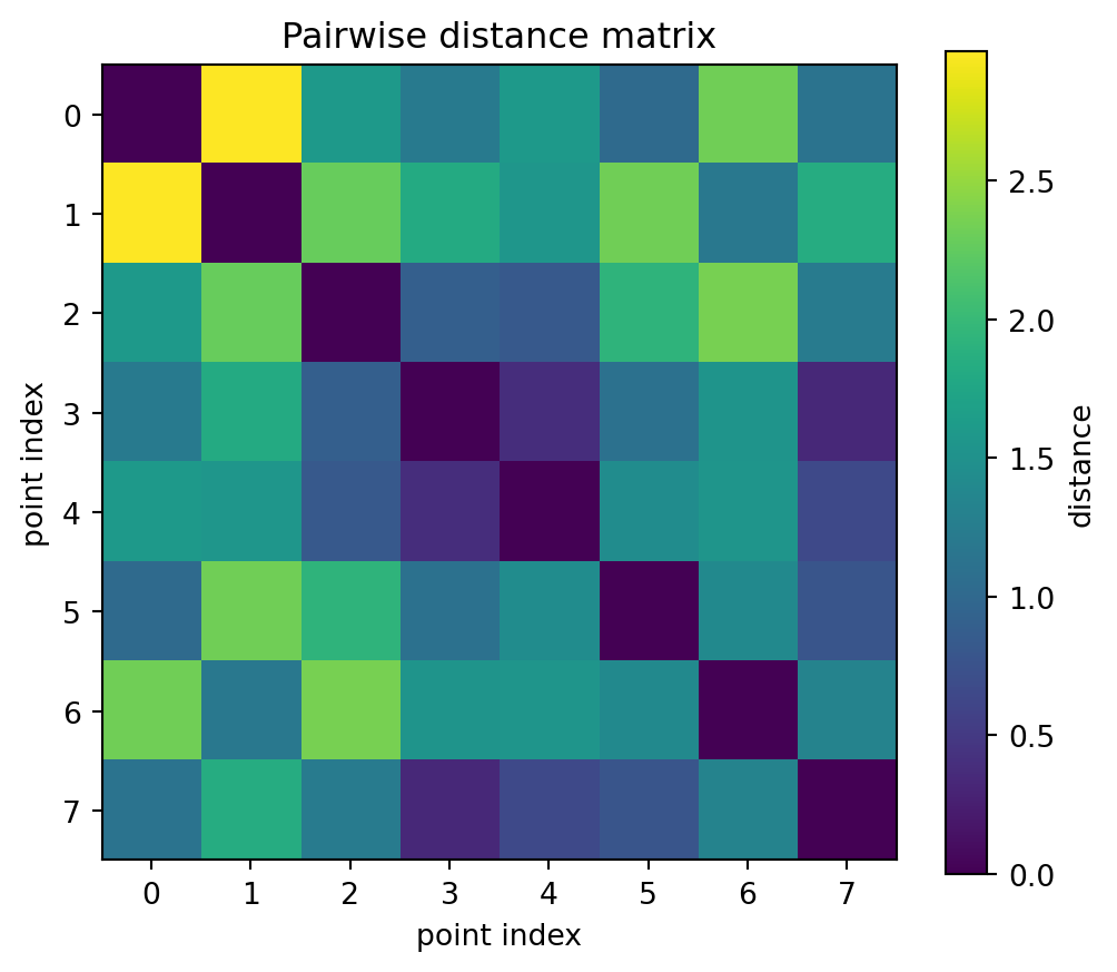
A distance matrix stores the distance between every pair of points in a dataset.
```{python}
np.random.seed(10)
X = np.random.normal(size=(8, 2))
D = pairwise_distances(X)

plt.figure(figsize=(6, 5))
plt.imshow(D)
plt.colorbar(label="distance")
plt.title("Pairwise distance matrix")
plt.xlabel("point index")
plt.ylabel("point index")
plt.show()
```
The diagonal entries are zero because every point has distance zero from itself. The matrix is symmetric because $d(x,y)=d(y,x)$.
## 9.18 AI Companion Activities
Use an AI assistant as a study partner, not as a replacement for your own reasoning.
### Prompt 1: Explain the Ruler
Ask:
> Explain Euclidean norm, Manhattan norm, and maximum norm using one geometric example and one data science example.
Then check whether the examples use correct formulas.
### Prompt 2: Create Scaling Examples
Ask:
> Give me a dataset with two features where raw Euclidean distance gives a misleading nearest neighbor, but standardized distance gives a better one.
Then compute the distances yourself in Python.
### Prompt 3: Debug Distance Code
Ask:
> Here is my Python function for pairwise distances. Find the bug and explain it.
Then paste your code and verify the correction.
### Prompt 4: High-Dimensional Reflection
Ask:
> Why can nearest-neighbor intuition become difficult in high-dimensional spaces? Explain without advanced probability.
Then write your own two-paragraph summary.
## 9.19 Summary
In this chapter, we learned how to measure size and difference in vector spaces.
The main ideas are:
- A norm measures the length or size of a vector.
- Euclidean length generalizes the Pythagorean theorem.
- Distance between points is the length of their difference.
- Error vectors measure how far predictions are from truth.
- Squared error is the square of Euclidean length.
- Unit vectors preserve direction but remove magnitude.
- Feature scaling is essential when using distance on real data.
- Different distances encode different modeling choices.
- In high dimensions, distance behaves differently from our geometric intuition.
- Matrix transformations can preserve, stretch, shrink, or destroy distances.
::: {.callout-important}
## Closing Thought
A vector space without distance is a place where objects exist.
A vector space with distance is a place where objects can be compared.
That comparison is the beginning of geometry, statistics, machine learning, and optimization.
:::