---
title: "Chapter 15: Energy Landscapes"
subtitle: "Quadratic forms, symmetric matrices, and the geometry of optimization"
format:
html:
toc: true
toc-depth: 3
number-sections: true
code-fold: true
code-tools: true
jupyter: python3
---
# Chapter 15: Energy Landscapes
## Opening story: every algorithm is walking on a landscape
Imagine standing in a dark valley with only one instruction:
> Take a small step downhill.
You cannot see the whole landscape. You only know the local slope under your feet. If the ground is shaped like a smooth bowl, every downhill step brings you closer to the bottom. If the ground is shaped like a saddle, one direction may feel safe while another direction sends you away. If the ground is almost flat in one direction and very steep in another, progress becomes slow and unstable.
This is not only a story about mountains. It is also a story about modern computation.
In statistics, we minimize squared prediction error. In machine learning, we minimize loss functions. In physics, systems move toward lower energy. In data science, we often search for the best vector of parameters. Around many important points, a complicated function behaves approximately like a quadratic bowl, hill, or saddle.
Linear algebra gives us the language for this local geometry.
A symmetric matrix $A$ creates an energy function
$$
q(x)=x^T A x.
$$
This expression takes a vector $x$ and returns a number. That number may represent energy, cost, squared length, risk, variance, or curvature. The shape of the landscape is controlled by the eigenvalues and eigenvectors of $A$.
The central message of this chapter is:
> A symmetric matrix is not only a transformation. It is also a landscape.
Eigenvectors are the principal directions of the landscape. Eigenvalues tell how strongly the landscape curves in those directions. Positive eigenvalues make bowls. Negative eigenvalues make hills. Mixed signs make saddles. Zero eigenvalues create flat valleys.
This chapter connects geometry, optimization, least squares, stability, and machine learning.
## Learning goals
By the end of this chapter, you should be able to:
1. Explain what a quadratic form $q(x)=x^T A x$ measures.
2. Interpret symmetric matrices as energy landscapes.
3. Recognize bowls, hills, saddles, and flat valleys from eigenvalues.
4. Define positive definite, positive semidefinite, negative definite, and indefinite matrices.
5. Use completing the square and eigenvectors to understand quadratic functions.
6. Compute gradients and Hessians of quadratic functions.
7. Explain why positive definiteness matters for minimization.
8. Understand condition number as a measure of landscape difficulty.
9. Use Python to visualize quadratic surfaces, contours, gradient descent, and high-dimensional quadratic optimization.
## 15.1 From vectors to numbers
So far, many matrices have acted like machines that send vectors to vectors:
$$
A x = y.
$$
A quadratic form sends a vector to a number:
$$
q(x)=x^T A x.
$$
This is a two-step process:
1. The matrix transforms $x$ into $Ax$.
2. The dot product compares $x$ with $Ax$.
So
$$
x^T A x = x \cdot (Ax).
$$
This means a quadratic form measures how much the transformed vector $Ax$ points in the same direction as the original vector $x$.
### Example: a stretched squared length
Let
$$
A=\begin{bmatrix}3&0\\0&1\end{bmatrix},
\qquad
x=\begin{bmatrix}x_1\\x_2\end{bmatrix}.
$$
Then
$$
q(x)=x^T A x
=3x_1^2+x_2^2.
$$
This is like squared length, except the $x_1$ direction is weighted three times more strongly than the $x_2$ direction. Moving horizontally costs more energy than moving vertically.
### Why quadratic forms appear everywhere
Quadratic forms appear naturally because many quantities are built from squared sizes:
- squared distance: $\|x\|^2=x^T x$;
- weighted squared distance: $x^T A x$;
- least-squares error: $\|Ax-b\|^2$;
- variance of a projection: $w^T \Sigma w$;
- local approximation of a smooth function near a point;
- energy stored in a physical system.
The square is important. A squared quantity is usually nonnegative, smooth, and sensitive to large errors.
## 15.2 Symmetric matrices are the natural landscape matrices
For a general square matrix $A$, the expression $x^T A x$ only depends on the symmetric part of $A$.
The symmetric part of $A$ is
$$
S=\frac{A+A^T}{2}.
$$
Then
$$
x^T A x = x^T S x.
$$
Why? The skew-symmetric part does not contribute to the quadratic form.
::: {.callout-tip}
## Key idea
Quadratic landscapes are controlled by symmetric matrices.
Even if $A$ is not symmetric, the energy $x^T A x$ only sees the symmetric part $\frac{A+A^T}{2}$.
:::
### Proof sketch
Write
$$
A=\frac{A+A^T}{2}+\frac{A-A^T}{2}=S+K,
$$
where $S^T=S$ and $K^T=-K$. For any vector $x$,
$$
x^T K x = 0.
$$
Therefore
$$
x^T A x=x^T S x+x^T K x=x^T S x.
$$
This is why symmetric matrices are the main actors in this chapter.
## 15.3 Landscapes in two dimensions
A quadratic form in two variables has the general shape
$$
q(x,y)=a x^2+2bxy+c y^2.
$$
The corresponding symmetric matrix is
$$
A=\begin{bmatrix}a&b\\b&c\end{bmatrix}.
$$
The cross term $2bxy$ couples the two coordinates. It means the principal directions of the landscape may not align with the coordinate axes.
### Four basic shapes
| Eigenvalues of $A$ | Shape of $q(x)=x^T A x$ | Optimization meaning |
|---|---|---|
| both positive | bowl | strict minimum at $0$ |
| both negative | upside-down bowl | strict maximum at $0$ |
| one positive, one negative | saddle | unstable critical point |
| one positive, one zero | flat valley | many minimizers along a line |
The eigenvalues tell the type of shape. The eigenvectors tell the directions of the axes of the shape.
## 15.4 The spectral theorem as a landscape decoder
A symmetric matrix can be diagonalized using an orthonormal basis of eigenvectors. This is one of the most important facts in linear algebra.
If $A$ is symmetric, then
$$
A=Q\Lambda Q^T,
$$
where $Q$ is an orthogonal matrix and $\Lambda$ is diagonal:
$$
\Lambda=
\begin{bmatrix}
\lambda_1 & 0 & \cdots & 0\\
0 & \lambda_2 & \cdots & 0\\
\vdots & \vdots & \ddots & \vdots\\
0 & 0 & \cdots & \lambda_n
\end{bmatrix}.
$$
The columns of $Q$ are orthonormal eigenvectors. The numbers $\lambda_1,\ldots,\lambda_n$ are eigenvalues.
Now set
$$
z=Q^T x.
$$
Since $Q$ is orthogonal, this is just a rotation or reflection of coordinates. It does not distort lengths. In these new coordinates,
$$
q(x)=x^T A x=z^T \Lambda z
=\lambda_1 z_1^2+\lambda_2 z_2^2+\cdots+\lambda_n z_n^2.
$$
This formula is the landscape decoder.
::: {.callout-important}
## Landscape decoder
For a symmetric matrix $A$,
$$
x^T A x = \lambda_1 z_1^2+\cdots+\lambda_n z_n^2,
$$
where the $z_i$ coordinates are measured along the eigenvector directions.
Eigenvectors give directions. Eigenvalues give curvature.
:::
## 15.5 Positive definite matrices
A symmetric matrix $A$ is **positive definite** if
$$
x^T A x>0
$$
for every nonzero vector $x$.
Geometrically, this means the energy landscape is a bowl with a unique bottom at the origin.
A symmetric matrix is positive definite exactly when all its eigenvalues are positive.
### Positive semidefinite matrices
A symmetric matrix $A$ is **positive semidefinite** if
$$
x^T A x\ge 0
$$
for every vector $x$.
This allows flat directions. Some nonzero vectors may have zero energy.
A symmetric matrix is positive semidefinite exactly when all its eigenvalues are nonnegative.
### Indefinite matrices
A symmetric matrix is **indefinite** if the quadratic form is positive in some directions and negative in others. This happens when $A$ has both positive and negative eigenvalues.
Indefinite matrices produce saddle landscapes.
## 15.6 Quadratic functions with linear terms
Many optimization problems are not just $x^T A x$. They also include a linear term.
A general quadratic function has the form
$$
f(x)=\frac12 x^T A x-b^T x+c,
$$
where $A$ is symmetric.
The gradient is
$$
\nabla f(x)=Ax-b.
$$
The Hessian is
$$
\nabla^2 f(x)=A.
$$
The critical point satisfies
$$
Ax=b.
$$
This is a powerful connection:
> Solving a linear system is the same as finding the bottom of a quadratic bowl when $A$ is positive definite.
### Completing the square
If $A$ is positive definite and $x_*=A^{-1}b$, then
$$
f(x)=\frac12 (x-x_*)^T A (x-x_*)+\text{constant}.
$$
The point $x_*$ is the unique minimizer.
## 15.7 Least squares as an energy landscape
In least squares, we want to solve
$$
Ax\approx b.
$$
The error vector is
$$
r(x)=Ax-b.
$$
The squared error is
$$
E(x)=\|Ax-b\|^2.
$$
Expanding gives
$$
E(x)=x^T A^T A x-2(A^T b)^T x+b^T b.
$$
This is a quadratic function. Its Hessian is related to $A^T A$, which is always positive semidefinite.
The normal equations are
$$
A^T A x=A^T b.
$$
This means least squares finds the bottom of an energy landscape built from squared residuals.
## 15.8 Gradient descent on a quadratic bowl
Consider
$$
f(x)=\frac12 x^T A x-b^T x,
$$
where $A$ is positive definite. Gradient descent updates
$$
x_{k+1}=x_k-\alpha(Ax_k-b).
$$
Here $\alpha$ is the step size.
If $\alpha$ is too small, progress is slow. If $\alpha$ is too large, the method can oscillate or diverge.
The eigenvalues of $A$ control this behavior. Large eigenvalues correspond to steep directions. Small eigenvalues correspond to flat directions.
### Condition number
For a positive definite matrix, the condition number is
$$
\kappa(A)=\frac{\lambda_{\max}}{\lambda_{\min}}.
$$
If $\kappa(A)$ is close to $1$, the bowl is round and gradient descent behaves well.
If $\kappa(A)$ is large, the bowl is long and narrow. Gradient descent may zigzag and converge slowly.
::: {.callout-warning}
## Computational warning
A narrow bowl is not mathematically impossible, but it can be computationally difficult.
This is why scaling, normalization, preconditioning, and better optimization methods matter.
:::
## 15.9 Curvature and local approximation
For a smooth function $f(x)$, the second-order Taylor approximation near a point $x_0$ is
$$
f(x_0+h)\approx f(x_0)+\nabla f(x_0)^T h+\frac12 h^T H h,
$$
where $H$ is the Hessian matrix.
The quadratic term
$$
\frac12 h^T H h
$$
describes local curvature.
So even when the original function is not quadratic, its local behavior is often governed by a quadratic form.
This is why eigenvalues of Hessian matrices matter in optimization and machine learning.
## 15.10 Energy landscapes in machine learning
Many machine learning models are trained by minimizing a loss function. The loss function is an energy landscape over the parameter space.
For linear regression, the loss is a convex quadratic bowl:
$$
L(w)=\|Xw-y\|^2.
$$
For neural networks, the loss landscape is not globally quadratic. It may contain valleys, saddles, flat regions, and complicated curved structures. But locally, near a point, the Hessian still provides a quadratic approximation.
The linear algebra ideas in this chapter help explain:
- why some directions are steep and others are flat;
- why gradient descent can be slow in narrow valleys;
- why scaling features helps optimization;
- why positive definiteness gives unique minimizers;
- why saddle points are unstable;
- why second-order methods use curvature information.
## 15.11 Worked examples
### Example 1: classify the landscape
Let
$$
A=\begin{bmatrix}4&0\\0&1\end{bmatrix}.
$$
Then
$$
q(x,y)=4x^2+y^2.
$$
Both eigenvalues are positive, so the landscape is a bowl. The energy grows faster in the $x$ direction than in the $y$ direction.
### Example 2: a saddle
Let
$$
A=\begin{bmatrix}1&0\\0&-2\end{bmatrix}.
$$
Then
$$
q(x,y)=x^2-2y^2.
$$
The $x$ direction curves upward. The $y$ direction curves downward. The origin is a saddle point.
### Example 3: a rotated bowl
Let
$$
A=\begin{bmatrix}3&1\\1&3\end{bmatrix}.
$$
The eigenvectors are along the directions $(1,1)$ and $(1,-1)$. The eigenvalues are $4$ and $2$. Therefore the landscape is a bowl whose principal axes are rotated relative to the coordinate axes.
### Example 4: least squares landscape
Suppose
$$
A=\begin{bmatrix}1&1\\1&2\\1&3\end{bmatrix},
\qquad
b=\begin{bmatrix}1\\2\\2\end{bmatrix}.
$$
Least squares minimizes
$$
E(x)=\|Ax-b\|^2.
$$
The matrix controlling curvature is $A^T A$:
$$
A^T A=\begin{bmatrix}3&6\\6&14\end{bmatrix}.
$$
Since $A$ has independent columns, $A^T A$ is positive definite. Therefore the least-squares landscape is a bowl with a unique minimizer.
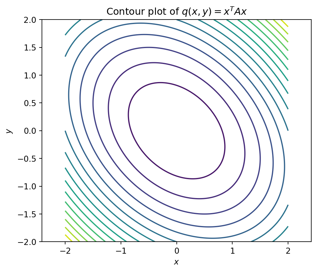
## 15.12 Python: visualizing bowls and saddles
```{python}
import numpy as np
import matplotlib.pyplot as plt

A = np.array([[3, 1], [1, 3]])

x = np.linspace(-2, 2, 200)
y = np.linspace(-2, 2, 200)
X, Y = np.meshgrid(x, y)
Z = A[0,0]*X**2 + 2*A[0,1]*X*Y + A[1,1]*Y**2

plt.figure(figsize=(6, 5))
plt.contour(X, Y, Z, levels=20)
plt.axis('equal')
plt.xlabel('$x$')
plt.ylabel('$y$')
plt.title('Contour plot of $q(x,y)=x^T A x$')
plt.show()
```
The contour plot shows level curves: curves where the energy has the same value. For a positive definite matrix, the contours are ellipses.
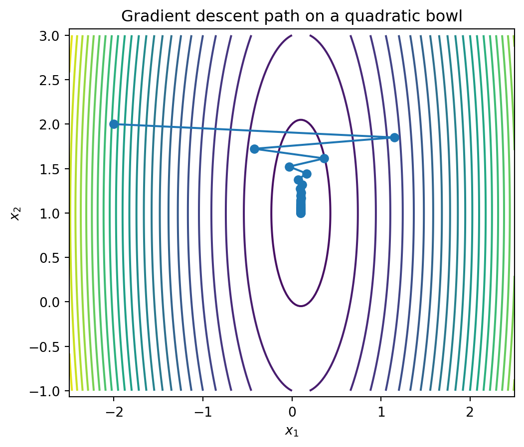
## 15.13 Python: gradient descent on a quadratic
```{python}
A = np.array([[10, 0], [0, 1]])
b = np.array([1, 1])
alpha = 0.15

x = np.array([-2.0, 2.0])
path = [x.copy()]

for k in range(40):
    grad = A @ x - b
    x = x - alpha * grad
    path.append(x.copy())

path = np.array(path)

xs = np.linspace(-2.5, 2.5, 200)
ys = np.linspace(-1, 3, 200)
X, Y = np.meshgrid(xs, ys)
Z = 0.5*(A[0,0]*X**2 + A[1,1]*Y**2) - b[0]*X - b[1]*Y

plt.figure(figsize=(6,5))
plt.contour(X, Y, Z, levels=25)
plt.plot(path[:,0], path[:,1], marker='o')
plt.axis('equal')
plt.xlabel('$x_1$')
plt.ylabel('$x_2$')
plt.title('Gradient descent path on a quadratic bowl')
plt.show()
```
The path moves downhill. If the bowl is narrow, the path may zigzag.
## 15.14 Practice problems
### Problem 1
For each matrix, classify the quadratic form as positive definite, negative definite, positive semidefinite, or indefinite.
$$
A_1=\begin{bmatrix}2&0\\0&5\end{bmatrix},
\qquad
A_2=\begin{bmatrix}1&0\\0&-1\end{bmatrix},
\qquad
A_3=\begin{bmatrix}1&1\\1&1\end{bmatrix}.
$$
::: {.callout-note collapse="true"}
## Solution
$A_1$ has eigenvalues $2$ and $5$, so it is positive definite.
$A_2$ has eigenvalues $1$ and $-1$, so it is indefinite.
$A_3$ has eigenvalues $2$ and $0$, so it is positive semidefinite.
:::
### Problem 2
Let
$$
A=\begin{bmatrix}2&1\\1&2\end{bmatrix}.
$$
Find the eigenvalues and describe the landscape of $q(x)=x^T A x$.
::: {.callout-note collapse="true"}
## Solution
The eigenvectors are $(1,1)$ and $(1,-1)$. The eigenvalues are $3$ and $1$. Both are positive, so the landscape is a rotated bowl. It is steeper in the $(1,1)$ direction.
:::
### Problem 3
For
$$
f(x)=\frac12 x^T A x-b^T x,
$$
show that $\nabla f(x)=Ax-b$ when $A$ is symmetric.
::: {.callout-note collapse="true"}
## Solution
The derivative of $\frac12 x^T A x$ is $\frac12(A+A^T)x$. If $A$ is symmetric, this becomes $Ax$. The derivative of $-b^T x$ is $-b$. Therefore $\nabla f(x)=Ax-b$.
:::
### Problem 4
Explain why the least-squares function
$$
E(x)=\|Ax-b\|^2
$$
has a positive semidefinite Hessian.
::: {.callout-note collapse="true"}
## Solution
Expanding gives
$$
E(x)=x^T A^T A x-2(A^T b)^T x+b^T b.
$$
The Hessian is $2A^T A$. For every vector $z$,
$$
z^T A^T A z=\|Az\|^2\ge 0.
$$
So $A^T A$ and $2A^T A$ are positive semidefinite.
:::
## 15.15 Challenge questions
1. Why do the contours of a positive definite quadratic form look like ellipses?
2. What happens to gradient descent when one eigenvalue is much larger than another?
3. Why does feature scaling improve optimization for linear regression?
4. How does a saddle point differ from a local minimum?
5. In high dimensions, why might a loss function have many flat directions?
## 15.16 AI companion activities
Use an AI assistant as a mathematical conversation partner.
1. Ask it to explain positive definite matrices using three metaphors: geometry, physics, and optimization.
2. Give it a $2\times2$ symmetric matrix and ask it to classify the landscape, then verify using eigenvalues.
3. Ask it to generate a contour plot for a quadratic form and explain the shape.
4. Ask it to compare gradient descent on a round bowl and a narrow bowl.
5. Ask it to explain how the Hessian matrix describes local curvature in machine learning.
## Chapter summary
A quadratic form $x^T A x$ turns a vector into a number. When $A$ is symmetric, this number defines an energy landscape. The spectral theorem reveals the hidden geometry: eigenvectors give the principal directions, and eigenvalues give the curvature in those directions.
Positive definite matrices create bowls with unique minima. Positive semidefinite matrices create bowls with flat directions. Indefinite matrices create saddles. These ideas explain least squares, optimization, gradient descent, numerical conditioning, and the local geometry of machine learning loss functions.
The next chapter will use this landscape viewpoint to understand one of the most powerful tools in linear algebra: the singular value decomposition.