---
title: "Chapter 21: Images as Matrices"
subtitle: "Pixels, channels, filters, and the linear algebra of vision"
format:
html:
toc: true
toc-depth: 3
number-sections: true
code-fold: true
code-tools: true
jupyter: python3
---
## Opening Story: Seeing with Numbers
When we look at a photograph, we see a face, a building, a handwritten digit, a medical scan, or a landscape.
A computer sees numbers.
A grayscale image is a rectangle of brightness values.
A color image is three rectangles of brightness values: red, green, and blue.
The beautiful idea is this:
> An image is a matrix, and image processing is linear algebra acting on that matrix.
This means that the same ideas we have studied throughout the book appear inside images:
- vectors,
- matrices,
- distance,
- projection,
- orthogonality,
- filters,
- compression,
- SVD,
- edges,
- noise,
- and features.
Images are one of the best places to see linear algebra because the result is visual.
When we change the numbers, the picture changes.
When we transform the matrix, the image changes.
When we compress the matrix, the image loses detail.
When we apply a filter, edges and patterns appear.
The central idea of this chapter is:
> Computer vision begins by treating images as numerical arrays.
This chapter connects linear algebra to images, data science, and AI.
## Learning Goals
By the end of this chapter, you should be able to:
1. Understand a grayscale image as a matrix of pixel values.
2. Understand a color image as three matrices or a three-dimensional array.
3. Interpret pixels as coordinates of visual information.
4. Use Python to create, display, and manipulate simple images.
5. Understand brightness, contrast, thresholding, and inversion.
6. Understand image filters as local matrix operations.
7. Explain edge detection using differences.
8. Understand convolution as sliding a small matrix across an image.
9. Connect images to vectors, features, SVD, and AI.
10. See computer vision as linear algebra on image data.
## 21.1 A Grayscale Image Is a Matrix
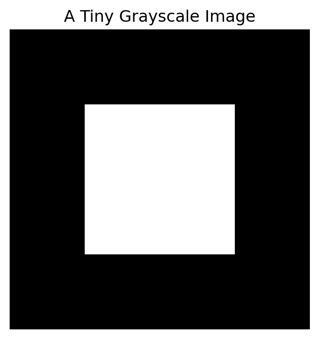
A grayscale image is a matrix.
Each entry is a pixel brightness.
For example,
$$
A =
\begin{bmatrix}
0 & 0 & 0 & 0 \\
0 & 1 & 1 & 0 \\
0 & 1 & 1 & 0 \\
0 & 0 & 0 & 0
\end{bmatrix}
$$
can represent a small white square on a black background.
Here:
- $0$ means black,
- $1$ means white,
- values between $0$ and $1$ mean shades of gray.
::: {.callout-important}
## Main Idea
A grayscale image is a matrix.
The entry $a_{ij}$ gives the brightness of the pixel in row $i$ and column $j$.
:::
Let us create and display this tiny image.
```{python}
import numpy as np
import matplotlib.pyplot as plt

tiny = np.array([
    [0, 0, 0, 0],
    [0, 1, 1, 0],
    [0, 1, 1, 0],
    [0, 0, 0, 0]
], dtype=float)

plt.figure(figsize=(4, 4))
plt.imshow(tiny, cmap="gray", vmin=0, vmax=1)
plt.title("A Tiny Grayscale Image")
plt.axis("off")
plt.show()
```
The picture is just a visual display of the matrix.
## 21.2 Rows, Columns, and Pixels
An image matrix has rows and columns.
If an image has $m$ rows and $n$ columns, then it has
$$
m \times n
$$
pixels.
For example, a $1000 \times 800$ grayscale image has
$$
1000 \cdot 800 = 800{,}000
$$
pixels.
Each pixel is one number.
So the image is a point in a very high-dimensional space.
A $1000 \times 800$ grayscale image can be viewed as a vector in
$$
\mathbb{R}^{800000}.
$$
::: {.callout-note}
## Image as High-Dimensional Vector
An image with $m n$ grayscale pixels can be treated as a vector in $\mathbb{R}^{mn}$.
:::
This is one reason linear algebra is central to computer vision.
Images are high-dimensional data points.
## 21.3 Creating Simple Images in Python
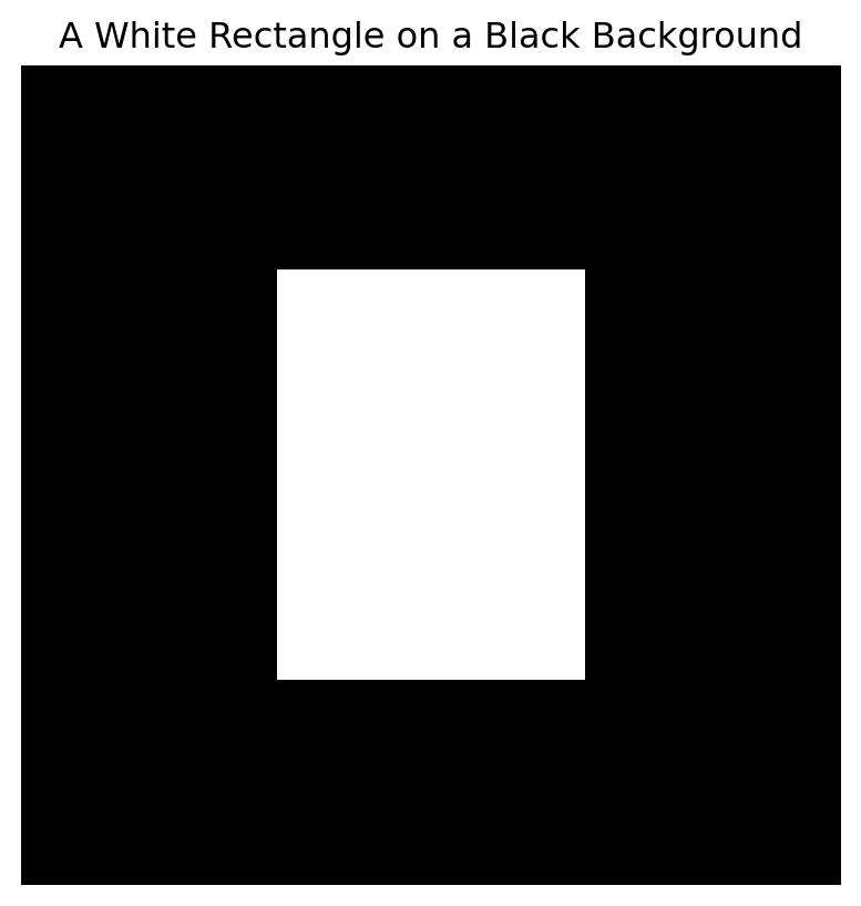
Let us create a larger image.
```{python}
image = np.zeros((80, 80))

image[20:60, 25:55] = 1.0

plt.figure(figsize=(5, 5))
plt.imshow(image, cmap="gray", vmin=0, vmax=1)
plt.title("A White Rectangle on a Black Background")
plt.axis("off")
plt.show()
```
The code
```python
image[20:60, 25:55] = 1.0
```
sets rows $20$ through $59$ and columns $25$ through $54$ to white.
This creates a rectangle.
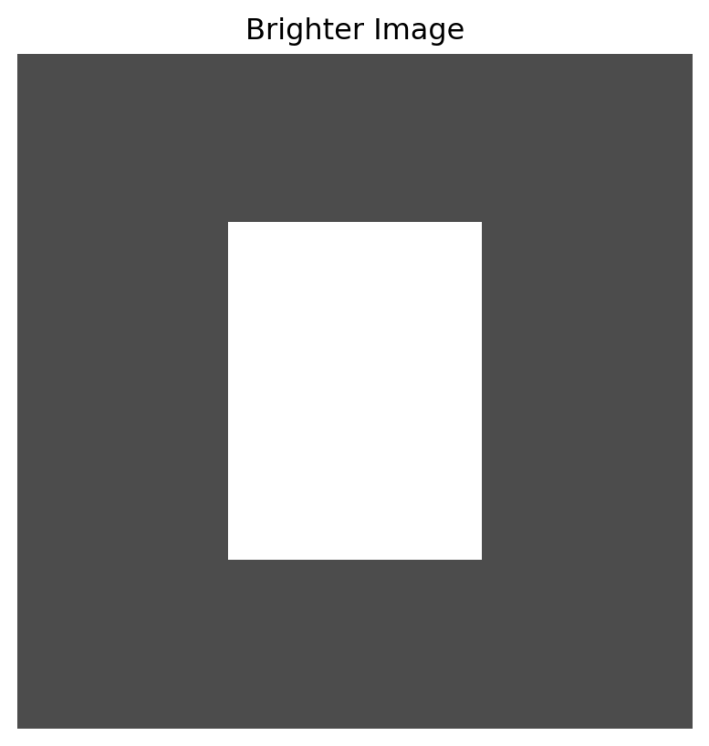
## 21.4 Brightness
Increasing brightness means adding a positive number to pixel values.
If $A$ is an image matrix, then
$$
A_{\text{bright}} = A + c
$$
makes the image brighter.
We usually clip values so they stay between $0$ and $1$.
```{python}
bright = np.clip(image + 0.3, 0, 1)

plt.figure(figsize=(5, 5))
plt.imshow(bright, cmap="gray", vmin=0, vmax=1)
plt.title("Brighter Image")
plt.axis("off")
plt.show()
```
This is a simple matrix operation.
Every pixel receives the same shift.
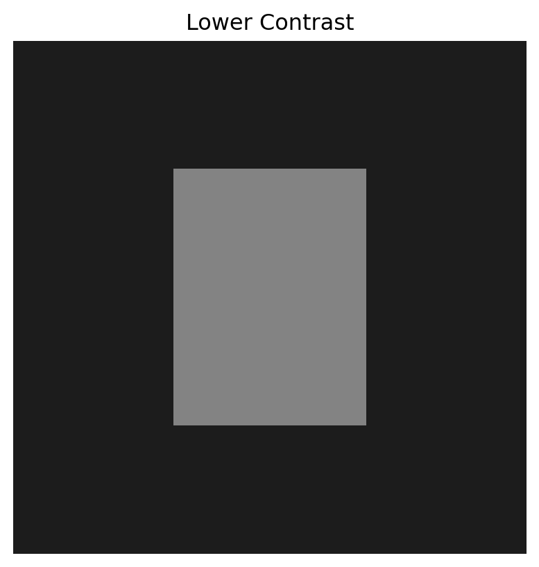
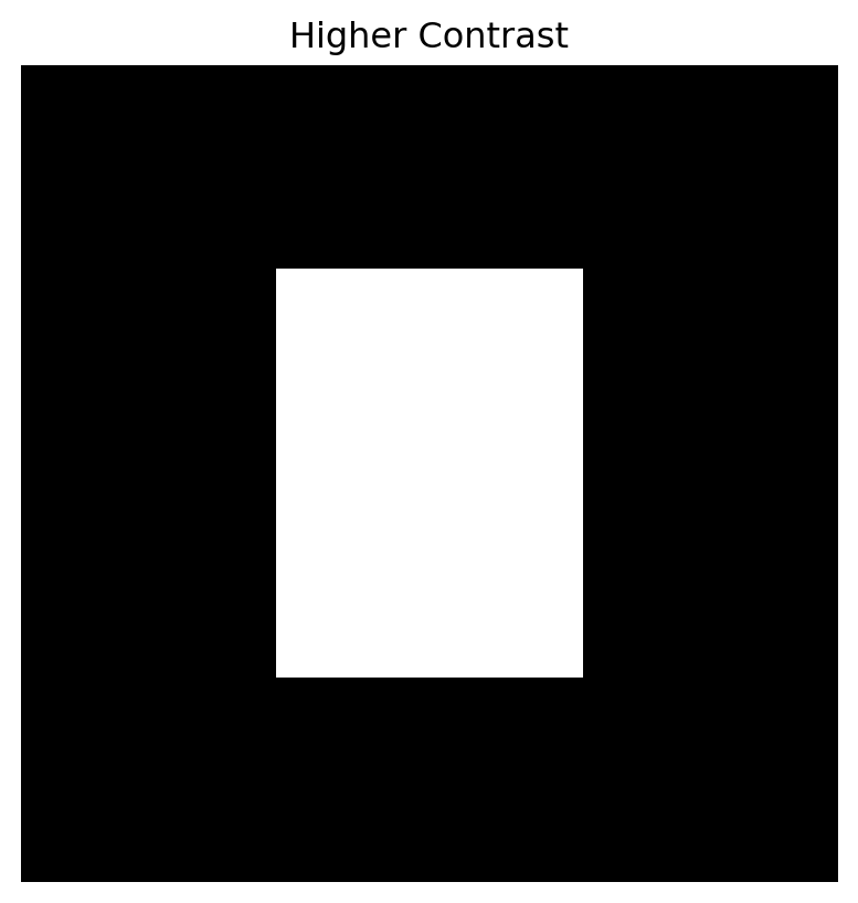
## 21.5 Contrast
Contrast controls how different dark and bright pixels are.
One simple contrast change is
$$
A_{\text{contrast}} = c(A-\bar{A})+\bar{A},
$$
where $\bar{A}$ is the average pixel value.
If $c>1$, contrast increases.
If $0<c<1$, contrast decreases.
```{python}
mean_value = image.mean()

high_contrast = np.clip(2.0 * (image - mean_value) + mean_value, 0, 1)
low_contrast = np.clip(0.4 * (image - mean_value) + mean_value, 0, 1)

plt.figure(figsize=(5, 5))
plt.imshow(low_contrast, cmap="gray", vmin=0, vmax=1)
plt.title("Lower Contrast")
plt.axis("off")
plt.show()

plt.figure(figsize=(5, 5))
plt.imshow(high_contrast, cmap="gray", vmin=0, vmax=1)
plt.title("Higher Contrast")
plt.axis("off")
plt.show()
```
Brightness adds.
Contrast stretches away from the mean.
Both are simple transformations of pixel values.
## 21.6 Image Inversion
An inverted grayscale image replaces each value by
$$
1-a_{ij}.
$$
So black becomes white, and white becomes black.
```{python}
inverted = 1 - image

plt.figure(figsize=(5, 5))
plt.imshow(inverted, cmap="gray", vmin=0, vmax=1)
plt.title("Inverted Image")
plt.axis("off")
plt.show()
```
Inversion is another pointwise transformation.
It acts on each pixel independently.
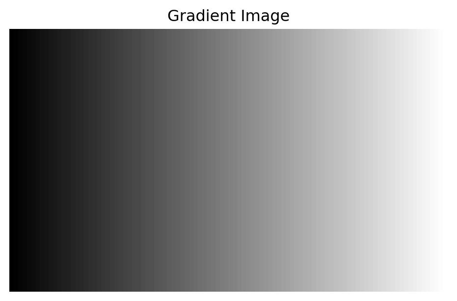
## 21.7 Thresholding
Thresholding turns a grayscale image into a black-and-white image.
Choose a threshold $t$.
Define
$$
b_{ij} =
\begin{cases}
1, & a_{ij} \geq t, \\
0, & a_{ij} < t.
\end{cases}
$$
This is useful when we want to separate foreground from background.
```{python}
gradient = np.tile(np.linspace(0, 1, 100), (60, 1))

threshold = 0.5
binary = (gradient >= threshold).astype(float)

plt.figure(figsize=(6, 4))
plt.imshow(gradient, cmap="gray", vmin=0, vmax=1)
plt.title("Gradient Image")
plt.axis("off")
plt.show()

plt.figure(figsize=(6, 4))
plt.imshow(binary, cmap="gray", vmin=0, vmax=1)
plt.title("Thresholded Image")
plt.axis("off")
plt.show()
```
Thresholding is simple but powerful.
It is often used in image segmentation.
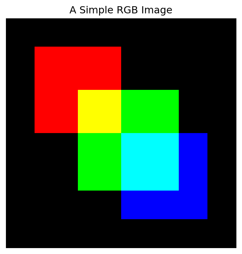
## 21.8 Color Images
A color image usually has three channels:
- red,
- green,
- blue.
Each channel is a matrix.
A color image can be represented as a three-dimensional array:
$$
m \times n \times 3.
$$
The first layer stores red values.
The second layer stores green values.
The third layer stores blue values.
::: {.callout-important}
## Color Image
A color image is often stored as three matrices:
$$
A_R,\quad A_G,\quad A_B.
$$
Together they form an RGB image.
:::
Let us create a simple color image.
```{python}
color = np.zeros((80, 80, 3))

# red square
color[10:40, 10:40, 0] = 1.0

# green square
color[25:60, 25:60, 1] = 1.0

# blue square
color[40:70, 40:70, 2] = 1.0

plt.figure(figsize=(5, 5))
plt.imshow(color)
plt.title("A Simple RGB Image")
plt.axis("off")
plt.show()
```
The color image is still numerical data.
It is just more structured than a grayscale matrix.
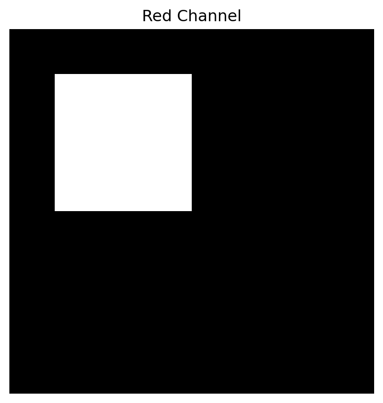
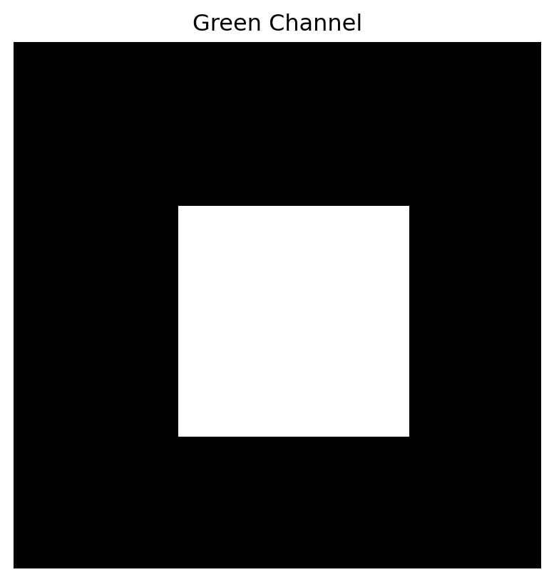
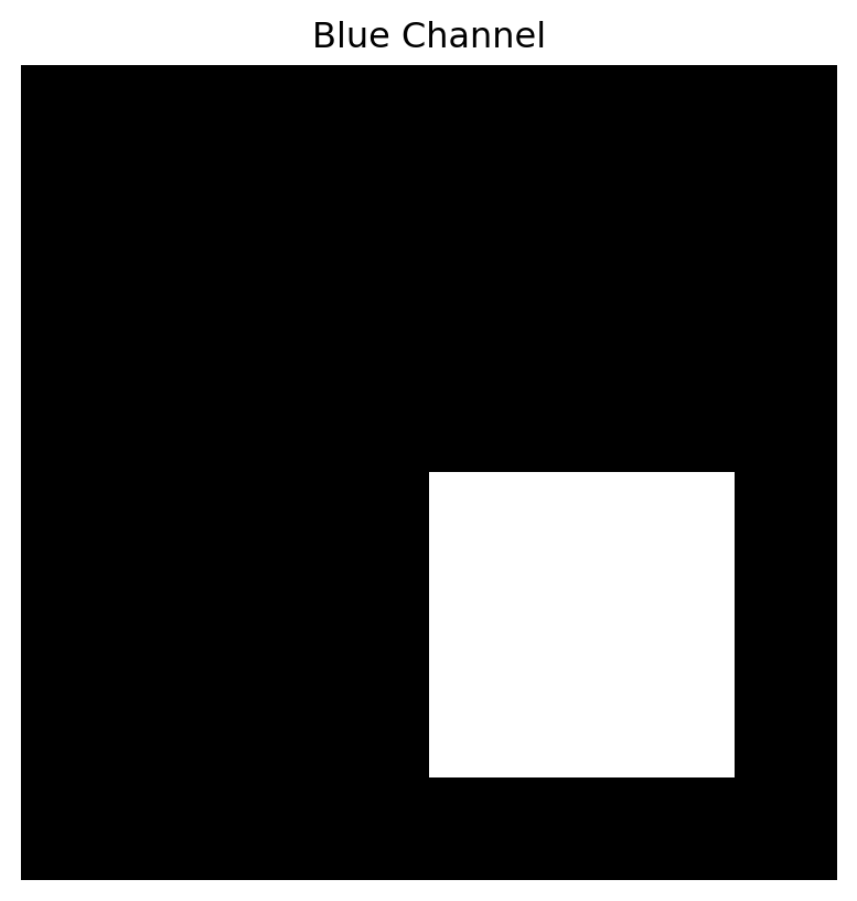
## 21.9 Separating Color Channels
We can display each channel separately.
```{python}
red = color[:, :, 0]
green = color[:, :, 1]
blue = color[:, :, 2]

for channel, name in [(red, "Red Channel"), (green, "Green Channel"), (blue, "Blue Channel")]:
    plt.figure(figsize=(5, 5))
    plt.imshow(channel, cmap="gray", vmin=0, vmax=1)
    plt.title(name)
    plt.axis("off")
    plt.show()
```
Each channel is a grayscale image.
Color comes from combining the three channels.
## 21.10 Flattening an Image into a Vector
Machine learning models often require data as vectors.
A grayscale image matrix can be flattened into a long vector.
If
$$
A \in \mathbb{R}^{m \times n},
$$
then flattening gives a vector in
$$
\mathbb{R}^{mn}.
$$
```{python}
flat = image.reshape(-1)

image.shape, flat.shape
```
This flattened vector can be used as a feature vector.
For example, handwritten digit images are often represented this way in simple machine learning models.
::: {.callout-note}
## Flattening
Flattening turns an image matrix into a long vector.
This makes images compatible with many data science algorithms.
:::
The drawback is that flattening may hide spatial structure.
Neighboring pixels in the image may no longer look like neighbors in the vector.
## 21.11 Distance Between Images
If images are vectors, we can compute distances between them.
For two images $A$ and $B$ of the same size, one distance is
$$
\|A-B\|_F,
$$
the Frobenius norm of the difference.
This is the square root of the sum of squared pixel differences:
$$
\|A-B\|_F =
\sqrt{
\sum_{i,j}(a_{ij}-b_{ij})^2
}.
$$
```{python}
image1 = np.zeros((80, 80))
image1[20:60, 25:55] = 1.0

image2 = np.zeros((80, 80))
image2[22:62, 27:57] = 1.0

distance = np.linalg.norm(image1 - image2, ord="fro")

distance
```
Distance gives one way to compare images.
But pixel distance may not always match human visual similarity.
Small shifts can create large pixel differences.
This is one reason image understanding is difficult.
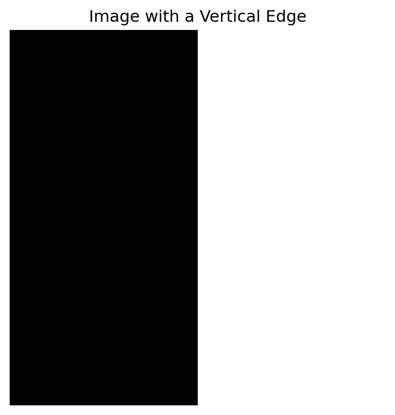
## 21.12 Local Differences
Edges are places where pixel values change quickly.
A simple horizontal difference is
$$
D_x(i,j)=A(i,j+1)-A(i,j).
$$
A simple vertical difference is
$$
D_y(i,j)=A(i+1,j)-A(i,j).
$$
These differences measure local change.
Let us create an image with an edge.
```{python}
edge_image = np.zeros((80, 80))
edge_image[:, 40:] = 1.0

plt.figure(figsize=(5, 5))
plt.imshow(edge_image, cmap="gray", vmin=0, vmax=1)
plt.title("Image with a Vertical Edge")
plt.axis("off")
plt.show()
```
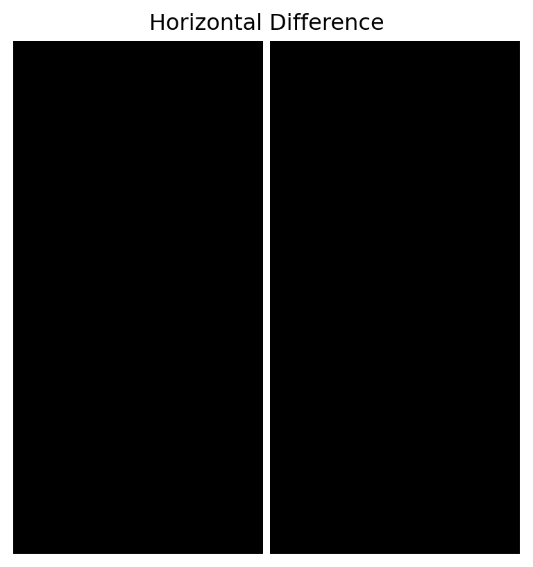
Compute horizontal differences.
```{python}
horizontal_diff = edge_image[:, 1:] - edge_image[:, :-1]

plt.figure(figsize=(5, 5))
plt.imshow(horizontal_diff, cmap="gray")
plt.title("Horizontal Difference")
plt.axis("off")
plt.show()
```
The difference is nonzero at the edge.
This is the simplest form of edge detection.
## 21.13 Filters as Small Matrices
An image filter applies a small matrix, called a kernel, to local neighborhoods of the image.
For example, a simple blur kernel is
$$
K =
\frac{1}{9}
\begin{bmatrix}
1 & 1 & 1 \\
1 & 1 & 1 \\
1 & 1 & 1
\end{bmatrix}.
$$
This replaces each pixel by the average of itself and its neighbors.
An edge-detection kernel might be
$$
K =
\begin{bmatrix}
-1 & 0 & 1
\end{bmatrix}.
$$
This measures horizontal change.
::: {.callout-important}
## Image Filter
An image filter uses a small matrix to combine nearby pixel values.
Filters can blur, sharpen, detect edges, or enhance patterns.
:::
## 21.14 Convolution: Sliding a Kernel
Convolution means sliding a kernel across an image.
At each location:
1. place the kernel over nearby pixels,
2. multiply corresponding entries,
3. add the results,
4. store the output.
For a $3 \times 3$ kernel, the output at a pixel depends on a $3 \times 3$ neighborhood.
This is a local linear operation.
::: {.callout-note}
## Convolution
Convolution is a local weighted sum operation.
It is one of the most important operations in image processing and computer vision.
:::
Let us implement a simple convolution.
```{python}
def convolve2d_simple(A, K):
    A = np.array(A, dtype=float)
    K = np.array(K, dtype=float)

    kh, kw = K.shape
    pad_h = kh // 2
    pad_w = kw // 2

    padded = np.pad(A, ((pad_h, pad_h), (pad_w, pad_w)), mode="edge")
    output = np.zeros_like(A)

    for i in range(A.shape[0]):
        for j in range(A.shape[1]):
            region = padded[i:i+kh, j:j+kw]
            output[i, j] = np.sum(region * K)

    return output
```
## 21.15 Blurring an Image
Use the averaging kernel.
```{python}
K_blur = np.ones((3, 3)) / 9

blurred = convolve2d_simple(edge_image, K_blur)

plt.figure(figsize=(5, 5))
plt.imshow(blurred, cmap="gray", vmin=0, vmax=1)
plt.title("Blurred Image")
plt.axis("off")
plt.show()
```
The edge becomes softer.
Blurring replaces each pixel by a local average.
## 21.16 Edge Detection with a Kernel
Use a horizontal difference kernel.
```{python}
K_edge = np.array([
    [-1, 0, 1]
], dtype=float)

edges = convolve2d_simple(edge_image, K_edge)

plt.figure(figsize=(5, 5))
plt.imshow(edges, cmap="gray")
plt.title("Edge Detection Kernel")
plt.axis("off")
plt.show()
```
The output highlights where the image changes horizontally.
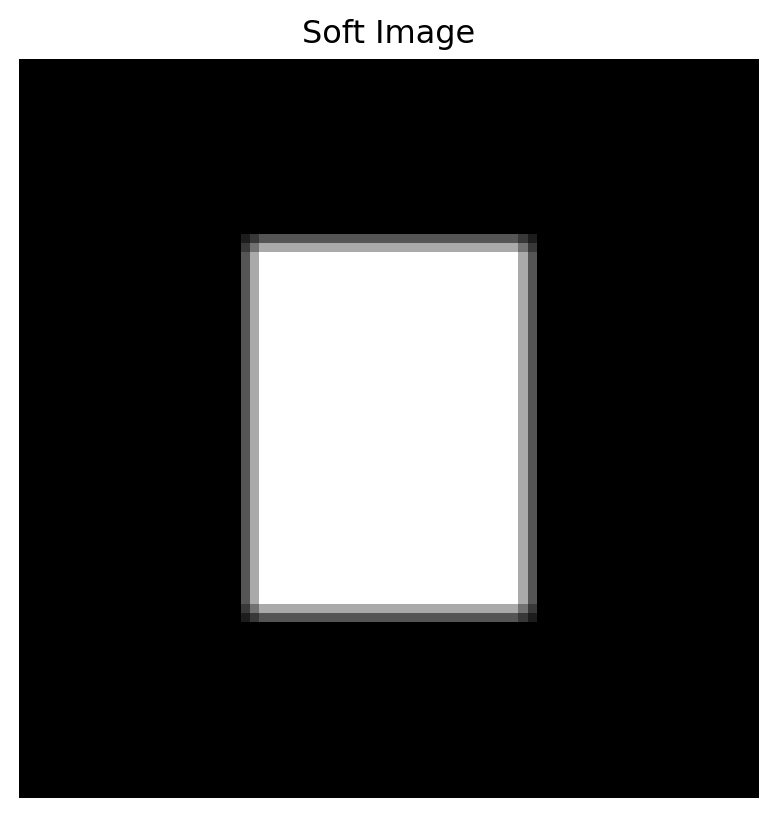
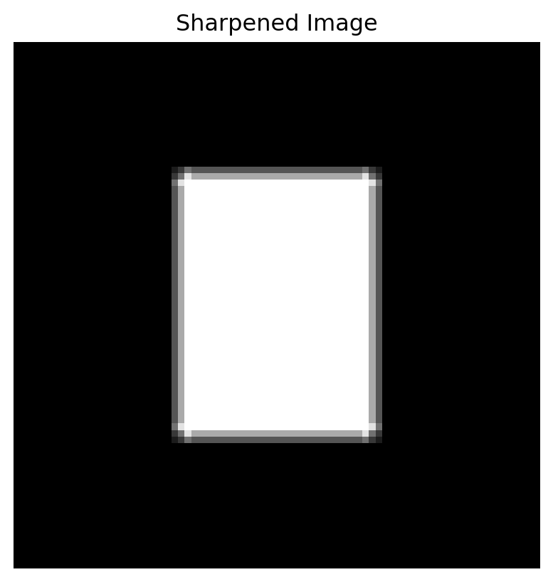
## 21.17 Sharpening
A sharpening filter can emphasize differences between a pixel and its neighbors.
One common sharpening kernel is
$$
K =
\begin{bmatrix}
0 & -1 & 0 \\
-1 & 5 & -1 \\
0 & -1 & 0
\end{bmatrix}.
$$
```{python}
soft_image = convolve2d_simple(image, K_blur)

K_sharp = np.array([
    [0, -1, 0],
    [-1, 5, -1],
    [0, -1, 0]
], dtype=float)

sharpened = np.clip(convolve2d_simple(soft_image, K_sharp), 0, 1)

plt.figure(figsize=(5, 5))
plt.imshow(soft_image, cmap="gray", vmin=0, vmax=1)
plt.title("Soft Image")
plt.axis("off")
plt.show()

plt.figure(figsize=(5, 5))
plt.imshow(sharpened, cmap="gray", vmin=0, vmax=1)
plt.title("Sharpened Image")
plt.axis("off")
plt.show()
```
Sharpening tries to restore or emphasize edges.
## 21.18 Filters and Linear Algebra
A filter is local, but it is still linear.
If $F$ is a filter operation, then
$$
F(A+B)=F(A)+F(B),
$$
and
$$
F(cA)=cF(A).
$$
So filtering is a linear transformation on image matrices.
If we flatten images into long vectors, a filter can be represented by a large matrix.
For an image with many pixels, this matrix is huge, but it has a repeated sparse structure.
::: {.callout-important}
## Filter as Linear Transformation
An image filter is a linear transformation.
It can be viewed as multiplying the flattened image vector by a large structured matrix.
:::
This connects convolution to linear algebra directly.
## 21.19 Convolution and Neural Networks
Convolution is central in computer vision and deep learning.
A convolutional neural network, or CNN, applies many learned filters to an image.
Early filters may detect:
- edges,
- corners,
- simple textures,
- light-dark contrasts.
Later layers combine these features into more complex patterns.
In a CNN, the filter entries are learned from data.
But the basic operation is still local weighted summation.
This is the same mathematical idea as convolution.
::: {.callout-note}
## AI Connection
A CNN learns filters that detect useful visual patterns.
The filter operation is a local linear transformation followed by nonlinear steps.
:::
## 21.20 Images and SVD
SVD can decompose an image matrix into layers.
As we saw in Chapter 17,
$$
A =
\sigma_1u_1v_1^T+
\sigma_2u_2v_2^T+
\cdots.
$$
The first layers capture large-scale structure.
Later layers capture smaller details.
Keeping the first $k$ layers gives a compressed image.
This shows another way matrices help us understand images.
Filters analyze local structure.
SVD analyzes global low-rank structure.
Both are useful.
## 21.21 Images and PCA
If we have many images of the same size, we can flatten each image into a vector.
Then the dataset becomes a matrix:
- rows are images,
- columns are pixels.
PCA can find directions of variation among images.
For example, in a face dataset, PCA may find patterns related to lighting, pose, expression, and shape.
These principal directions are sometimes called eigenfaces.
In beginner language:
> PCA finds common ways images vary across a dataset.
## 21.22 Images as Data for AI
Modern AI systems often treat images as tensors.
A grayscale image is like an $m \times n$ array.
A color image is like an $m \times n \times 3$ array.
A batch of images is like a larger array:
$$
N \times m \times n \times 3.
$$
Here $N$ is the number of images.
Deep learning systems use many operations on these arrays:
- convolution,
- matrix multiplication,
- normalization,
- pooling,
- nonlinear activation,
- attention,
- projection,
- embedding.
Linear algebra is not the whole story, but it is the foundation.
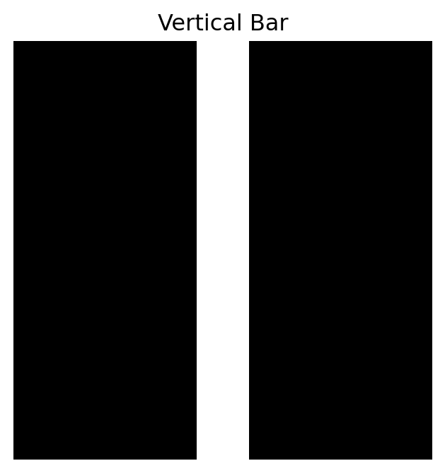
## 21.23 A Mini Image Classification Idea
Suppose we have two simple types of images:
- vertical bars,
- horizontal bars.
Each image can be flattened into a vector.
Then classification becomes a problem of comparing vectors.
Let us build a tiny dataset.
```{python}
def make_vertical_bar(size=16, col=7):
    A = np.zeros((size, size))
    A[:, col:col+2] = 1.0
    return A

def make_horizontal_bar(size=16, row=7):
    A = np.zeros((size, size))
    A[row:row+2, :] = 1.0
    return A

vertical = make_vertical_bar()
horizontal = make_horizontal_bar()

plt.figure(figsize=(4, 4))
plt.imshow(vertical, cmap="gray", vmin=0, vmax=1)
plt.title("Vertical Bar")
plt.axis("off")
plt.show()

plt.figure(figsize=(4, 4))
plt.imshow(horizontal, cmap="gray", vmin=0, vmax=1)
plt.title("Horizontal Bar")
plt.axis("off")
plt.show()
```
Flatten and compare a new image.
```{python}
new_image = make_vertical_bar(col=8)

v_vec = vertical.reshape(-1)
h_vec = horizontal.reshape(-1)
new_vec = new_image.reshape(-1)

dist_to_vertical = np.linalg.norm(new_vec - v_vec)
dist_to_horizontal = np.linalg.norm(new_vec - h_vec)

dist_to_vertical, dist_to_horizontal
```
The new image is closer to the vertical prototype.
This is a very simple classification idea.
Modern image classifiers are much more powerful, but the beginning is still representation and comparison.
## 21.24 Why Images Are Difficult
Images are high-dimensional.
A small $224 \times 224$ color image has
$$
224 \cdot 224 \cdot 3 = 150{,}528
$$
numbers.
But the difficulty is not only the number of pixels.
Images are difficult because:
- objects can move,
- lighting can change,
- scale can change,
- backgrounds vary,
- small rotations matter,
- important patterns are local,
- meaning depends on spatial relationships.
Linear algebra helps build tools for handling these challenges, but computer vision also needs statistics, optimization, and learning.
## 21.25 Concept Summary
A grayscale image is a matrix.
A color image is three matrices.
Pixel values are numerical data.
Simple image operations such as brightness, contrast, inversion, and thresholding act on pixel values.
Local differences detect edges.
Filters use small matrices called kernels.
Convolution slides a kernel across an image and computes local weighted sums.
Filtering is a linear transformation.
CNNs learn filters for visual tasks.
SVD compresses image matrices.
PCA studies variation across image datasets.
The main lesson is:
> Images are visual objects, but computers process them as numerical arrays.
## 21.26 Key Vocabulary
**Pixel**
One small unit of an image.
**Grayscale image**
An image represented by one brightness value per pixel.
**Image matrix**
A matrix of pixel values.
**RGB image**
A color image represented by red, green, and blue channels.
**Channel**
One color layer of an image.
**Flattening**
Turning an image matrix into a long vector.
**Thresholding**
Turning grayscale values into binary values using a cutoff.
**Filter**
A local operation that combines nearby pixel values.
**Kernel**
The small matrix used by a filter.
**Convolution**
Sliding a kernel across an image and computing weighted sums.
**Edge detection**
Finding locations where pixel values change sharply.
**CNN**
Convolutional neural network, a model that learns filters for images.
## 21.27 Practice Problems
### Problem 1
A grayscale image has size $300 \times 400$.
How many pixel values does it contain?
### Problem 2
A color RGB image has size $300 \times 400$.
How many numerical values does it contain?
### Problem 3
Explain why a grayscale image can be viewed as a vector.
### Problem 4
Given
$$
A =
\begin{bmatrix}
0 & 0 & 0 \\
0 & 1 & 1 \\
0 & 1 & 1
\end{bmatrix},
$$
compute the inverted image $1-A$.
### Problem 5
What does thresholding do?
Give a simple example.
### Problem 6
Why do local differences detect edges?
### Problem 7
Explain convolution in your own words.
### Problem 8
How is a filter a linear transformation?
### Problem 9
What is the difference between SVD image compression and convolution filtering?
### Problem 10
Why are images important examples of high-dimensional data?
## 21.28 Python Practice
### Exercise 1
Create a grayscale image matrix.
```{python}
A = np.zeros((50, 50))
A[15:35, 20:30] = 1.0

plt.figure(figsize=(5, 5))
plt.imshow(A, cmap="gray", vmin=0, vmax=1)
plt.axis("off")
plt.show()
```
### Exercise 2
Invert the image.
```{python}
A_inv = 1 - A

plt.figure(figsize=(5, 5))
plt.imshow(A_inv, cmap="gray", vmin=0, vmax=1)
plt.axis("off")
plt.show()
```
### Exercise 3
Create a gradient and threshold it.
```{python}
gradient = np.tile(np.linspace(0, 1, 80), (50, 1))
binary = (gradient > 0.6).astype(float)

plt.figure(figsize=(6, 4))
plt.imshow(binary, cmap="gray", vmin=0, vmax=1)
plt.axis("off")
plt.show()
```
### Exercise 4
Apply a blur filter.
```{python}
K_blur = np.ones((3, 3)) / 9

blurred = convolve2d_simple(A, K_blur)

plt.figure(figsize=(5, 5))
plt.imshow(blurred, cmap="gray", vmin=0, vmax=1)
plt.axis("off")
plt.show()
```
### Exercise 5
Apply an edge filter.
```{python}
K_edge = np.array([
    [-1, 0, 1]
], dtype=float)

edges = convolve2d_simple(A, K_edge)

plt.figure(figsize=(5, 5))
plt.imshow(edges, cmap="gray")
plt.axis("off")
plt.show()
```
### Exercise 6
Flatten an image and compute its length.
```{python}
flat = A.reshape(-1)

flat.shape, np.linalg.norm(flat)
```
### Exercise 7
Compare two images by distance.
```{python}
B = np.zeros((50, 50))
B[16:36, 21:31] = 1.0

np.linalg.norm(A - B, ord="fro")
```
## 21.29 AI Companion Activities
### Activity 1: Image as Matrix
Ask an AI tool:
> Explain how a grayscale image is represented as a matrix of pixel values.
Then create your own $5 \times 5$ image matrix.
### Activity 2: RGB Channels
Ask:
> Explain how RGB images are represented as three matrices.
Then describe what happens if the red channel is increased.
### Activity 3: Convolution
Ask:
> Explain convolution in image processing using beginner-friendly language.
Then apply the explanation to a blur filter.
### Activity 4: Edge Detection
Ask:
> Explain why differences between neighboring pixels can detect edges.
Then create a small matrix with an edge and compute differences.
### Activity 5: CNN Connection
Ask:
> Explain how convolutional neural networks use filters to detect visual patterns.
Then summarize the answer in three sentences.
## 21.30 Reflection Questions
1. Why is an image a matrix?
2. What does each pixel value mean?
3. How is a color image different from a grayscale image?
4. What does it mean to flatten an image?
5. Why can image distance be computed using matrix norms?
6. Why do edges correspond to local changes?
7. What is the role of a kernel in filtering?
8. Why is convolution a local linear operation?
9. How do CNNs build on image filters?
10. Why are images a natural place to learn linear algebra?
## 21.31 Chapter Closing
In this chapter, we studied images as matrices.
A grayscale image is a matrix of pixel values.
A color image is three matrices.
Image processing is the art of transforming these numerical arrays.
Brightness, contrast, inversion, thresholding, filtering, edge detection, SVD compression, and PCA all use linear algebra ideas.
Convolution shows how local matrix operations can reveal visual structure.
CNNs build on this by learning filters from data.
The main lesson is:
> To a computer, vision begins as linear algebra on arrays of numbers.
In the next chapter, we will move from images to networks.
There, matrices will describe connections instead of pixels.