---
title: "Chapter 4: Data as Points"
subtitle: "Feature spaces, data clouds, and the geometry of information"
format:
html:
toc: true
toc-depth: 3
number-sections: true
code-fold: true
code-tools: true
jupyter: python3
---
## Opening Story: When a Table Becomes a Shape
A table of data can look ordinary.
| Person | Hours studied | Sleep hours | Exam score |
|---|---:|---:|---:|
| A | 2 | 7 | 70 |
| B | 5 | 6 | 85 |
| C | 1 | 8 | 65 |
| D | 7 | 5 | 92 |
At first, it seems like a list of facts.
But linear algebra teaches us to look again.
Each row is not just a row. It is a point:
$$
(2,7,70), \quad (5,6,85), \quad (1,8,65), \quad (7,5,92).
$$
Each column is not just a column. It is a feature measured across the group.
The table has become geometry.
If we choose two features, such as hours studied and exam score, the students become points in a plane. If we choose three features, they become points in three-dimensional space. If we choose one hundred features, they become points in $\mathbb{R}^{100}$.
We may not be able to draw $\mathbb{R}^{100}$, but we can still compute in it. We can measure distance. We can find neighbors. We can detect clusters. We can identify unusual points. We can search for hidden directions.
This is one of the central ideas of modern data science:
> **Data becomes geometry.**
In Chapter 1, we learned that the world can be represented by numbers.
In Chapter 2, we learned that vectors are numbers with meaning.
In Chapter 3, we learned that vectors can be combined.
In this chapter, we study many vectors at once.
A dataset is a cloud of points.
Linear algebra gives us the language to understand the cloud.
## Learning Goals
By the end of this chapter, you should be able to:
1. Interpret a dataset as a collection of vectors.
2. Explain what a feature space is.
3. Read a data matrix by rows and by columns.
4. Visualize small datasets as point clouds.
5. Recognize trends, clusters, gaps, and outliers.
6. Explain why high-dimensional data is natural.
7. Understand why scaling changes the geometry of data.
8. Compute mean vectors and centered data.
9. Use Python to create, visualize, and analyze simple data clouds.
10. Connect data clouds to later topics: distance, projection, least squares, PCA, classification, and machine learning.
## 4.1 One Object, One Vector
A single object can be described by a vector.
For example, a student may be represented by
$$
x=
\begin{bmatrix}
5 \\
7 \\
88
\end{bmatrix},
$$
where the coordinates mean
$$
\begin{bmatrix}
\text{hours studied} \\
\text{sleep hours} \\
\text{exam score}
\end{bmatrix}.
$$
This vector is not just three numbers. It is a compact description of one student.
The meaning of the vector depends on the meaning of the coordinates. If the coordinate order changes, the meaning changes.
::: {.callout-important}
## A vector is a description
A data vector is a list of features describing one object.
The coordinates are not anonymous. They are measurements, counts, ratings, labels, or encoded properties.
:::
### Example: A House Vector
A house might be represented by
$$
h=
\begin{bmatrix}
1800 \\
3 \\
2 \\
12 \\
650000
\end{bmatrix},
$$
where the coordinates mean
$$
\begin{bmatrix}
\text{square feet} \\
\text{bedrooms} \\
\text{bathrooms} \\
\text{distance to downtown in miles} \\
\text{price in dollars}
\end{bmatrix}.
$$
The vector is a small numerical portrait of the house.
### Example: A Song Vector
A song may be represented by audio features:
$$
s=
\begin{bmatrix}
\text{tempo} \\
\text{energy} \\
\text{danceability} \\
\text{loudness} \\
\text{acousticness}
\end{bmatrix}.
$$
Then songs that sound similar may appear close together in this feature space.
## 4.2 Many Objects, Many Vectors
Data rarely contains just one object.
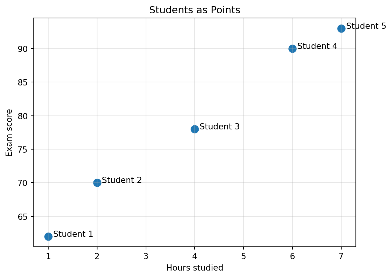
Suppose we have five students:
$$
x_1=
\begin{bmatrix}
1 \\
62
\end{bmatrix},
\quad
x_2=
\begin{bmatrix}
2 \\
70
\end{bmatrix},
\quad
x_3=
\begin{bmatrix}
4 \\
78
\end{bmatrix},
\quad
x_4=
\begin{bmatrix}
6 \\
90
\end{bmatrix},
\quad
x_5=
\begin{bmatrix}
7 \\
93
\end{bmatrix}.
$$
The first coordinate is hours studied. The second coordinate is exam score.
Each vector is one student.
Together, the vectors form a dataset.
::: {.callout-note}
## Dataset
A dataset is a collection of objects.
After we choose numerical features, the dataset becomes a collection of vectors.
:::
```{python}
import numpy as np
import matplotlib.pyplot as plt

X = np.array([
    [1, 62],
    [2, 70],
    [4, 78],
    [6, 90],
    [7, 93]
])

plt.figure(figsize=(7, 5))
plt.scatter(X[:, 0], X[:, 1], s=80)
for i, (a, b) in enumerate(X, start=1):
    plt.text(a + 0.1, b, f"Student {i}")
plt.xlabel("Hours studied")
plt.ylabel("Exam score")
plt.title("Students as Points")
plt.grid(True, alpha=0.3)
plt.show()
```
A small table has become a small picture.
The picture already says something: the cloud moves upward.
## 4.3 Feature Space
When we choose features, we create a coordinate system.
This coordinate system is called **feature space**.
If we choose two features, the feature space is two-dimensional. If we choose three features, it is three-dimensional. If we choose $n$ features, it is $\mathbb{R}^n$.
For example, the vector
$$
\begin{bmatrix}
\text{hours studied} \\
\text{exam score}
\end{bmatrix}
$$
lives in a two-dimensional feature space.
The vector
$$
\begin{bmatrix}
\text{hours studied} \\
\text{sleep hours} \\
\text{exam score}
\end{bmatrix}
$$
lives in a three-dimensional feature space.
A document represented by counts of 5000 words lives in $\mathbb{R}^{5000}$.
::: {.callout-important}
## Feature space
A feature space is the space whose coordinates are the features used to describe the objects.
In feature space, objects become points.
:::
### Why the Feature Choice Matters
The same object can live in different feature spaces depending on what we measure.
A restaurant could be represented by
$$
\begin{bmatrix}
\text{price} \\
\text{rating}
\end{bmatrix}
$$
or by
$$
\begin{bmatrix}
\text{price} \\
\text{rating} \\
\text{distance} \\
\text{noise level} \\
\text{number of vegetarian options}
\end{bmatrix}.
$$
The second representation may produce a very different geometry.
Two restaurants may be close using price and rating, but far apart after we include distance and menu type.
Feature choice is not a technical detail. It shapes the geometry of the problem.
## 4.4 Data Clouds
When many data points are plotted together, they form a **data cloud**.
The cloud may reveal structure:
- a **trend**, where points move in a general direction;
- a **cluster**, where points gather into groups;
- a **gap**, where few points appear;
- an **outlier**, where one point is far from the rest;
- a **curve**, where the structure is nonlinear;
- a **hidden direction**, where most variation happens along one line or plane.
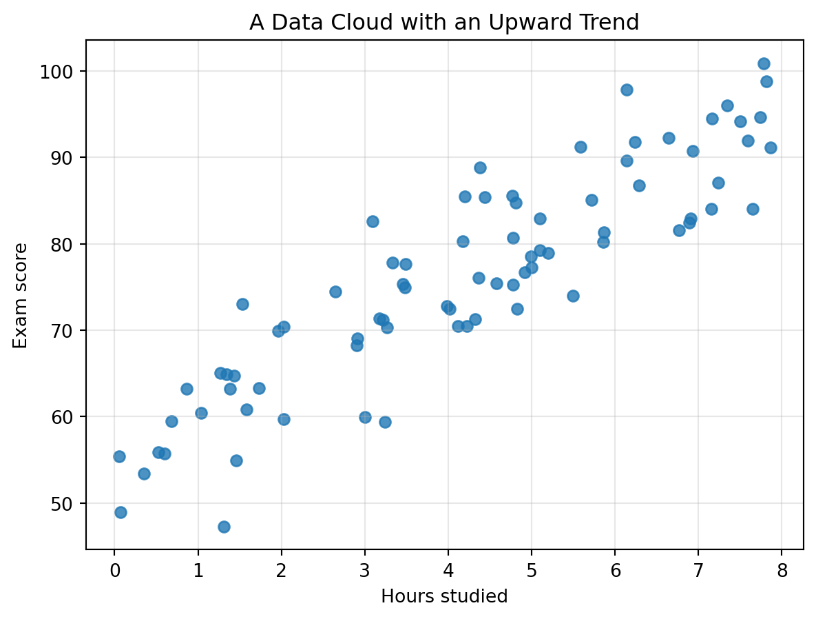
Let us create a synthetic example.
```{python}
np.random.seed(4)

hours = np.random.uniform(0, 8, 80)
scores = 55 + 5 * hours + np.random.normal(0, 6, size=80)

plt.figure(figsize=(7, 5))
plt.scatter(hours, scores, alpha=0.8)
plt.xlabel("Hours studied")
plt.ylabel("Exam score")
plt.title("A Data Cloud with an Upward Trend")
plt.grid(True, alpha=0.3)
plt.show()
```
The points are not exactly on a line.
But the cloud has a direction.
That direction is an important piece of information.
Later, we will learn methods that find such directions automatically.
## 4.5 The Data Matrix
A dataset is often stored as a matrix.
Suppose we measure four students using three features:
- hours studied,
- sleep hours,
- exam score.
| Student | Hours studied | Sleep hours | Exam score |
|---|---:|---:|---:|
| A | 2 | 7 | 70 |
| B | 5 | 6 | 85 |
| C | 1 | 8 | 65 |
| D | 7 | 5 | 92 |
The corresponding data matrix is
$$
X=
\begin{bmatrix}
2 & 7 & 70 \\
5 & 6 & 85 \\
1 & 8 & 65 \\
7 & 5 & 92
\end{bmatrix}.
$$
This is a $4 \times 3$ matrix.
It has 4 rows and 3 columns.
The common data science convention is:
$$
\text{rows} = \text{objects},
\qquad
\text{columns} = \text{features}.
$$
So this matrix represents 4 objects, each described by 3 features.
```{python}
X = np.array([
    [2, 7, 70],
    [5, 6, 85],
    [1, 8, 65],
    [7, 5, 92]
])

X.shape
```
The first row is the vector for Student A.
```{python}
X[0]
```
The third column is the exam score feature across all students.
```{python}
X[:, 2]
```
::: {.callout-tip}
## Shape of a data matrix
If $X$ has shape $m \times n$, then $X$ represents $m$ objects in $\mathbb{R}^n$.
Each row is one point in feature space.
:::
## 4.6 Row View and Column View
The same matrix has two useful readings.
### Row View: Objects
The row view reads each row as one object:
$$
X=
\begin{bmatrix}
\text{---} & x_1 & \text{---} \\
\text{---} & x_2 & \text{---} \\
\text{---} & x_3 & \text{---} \\
\text{---} & x_4 & \text{---}
\end{bmatrix}.
$$
This view asks:
> What is the complete description of one object?
In machine learning, the row view is often the view of examples, observations, customers, patients, images, houses, or documents.
### Column View: Features
The column view reads each column as one feature measured across all objects:
$$
X=
\begin{bmatrix}
| & | & | \\
\text{hours} & \text{sleep} & \text{score} \\
| & | & |
\end{bmatrix}.
$$
This view asks:
> How does one feature vary across the dataset?
The column view is essential for means, variances, correlations, and later for matrix transformations.
::: {.callout-note}
## Two meanings of the same matrix
Rows describe objects.
Columns describe features.
Good data analysis often moves between these two views.
:::
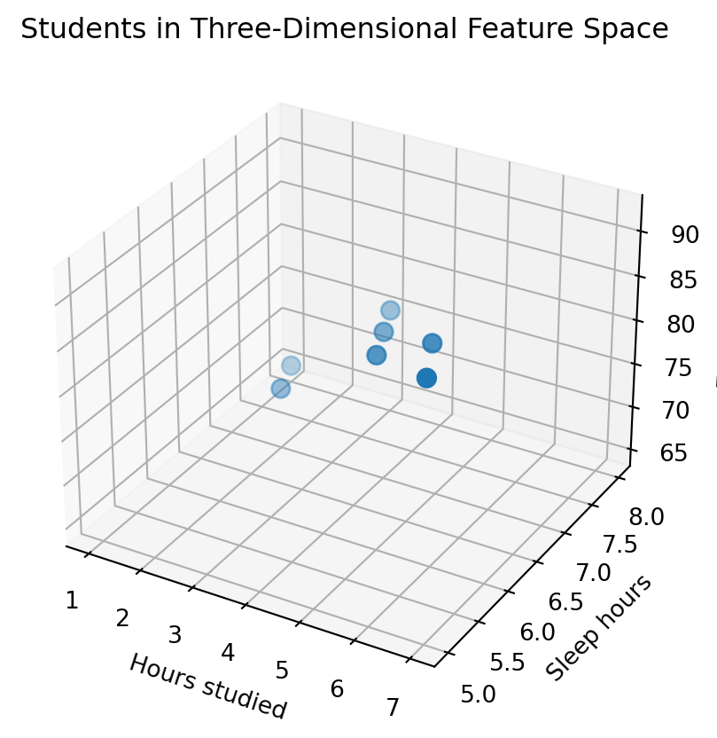
## 4.7 Three-Dimensional Data
If each object has three features, we can place each object in three-dimensional space.
For example, a student may be represented by
$$
\begin{bmatrix}
\text{hours studied} \\
\text{sleep hours} \\
\text{exam score}
\end{bmatrix}.
$$
```{python}
from mpl_toolkits.mplot3d import Axes3D  # noqa: F401

X3 = np.array([
    [2, 7, 70],
    [5, 6, 85],
    [1, 8, 65],
    [7, 5, 92],
    [4, 7, 80],
    [6, 6, 88],
    [3, 8, 75]
])

fig = plt.figure(figsize=(7, 5))
ax = fig.add_subplot(111, projection="3d")
ax.scatter(X3[:, 0], X3[:, 1], X3[:, 2], s=60)
ax.set_xlabel("Hours studied")
ax.set_ylabel("Sleep hours")
ax.set_zlabel("Exam score")
ax.set_title("Students in Three-Dimensional Feature Space")
plt.show()
```
Three-dimensional plots are useful, but they are already harder to read than two-dimensional plots.
Real datasets often have far more than three features.
This is why we need linear algebra: it lets us reason about spaces we cannot draw.
## 4.8 High-Dimensional Data Is Normal
High-dimensional data sounds advanced, but it is everywhere.
A grayscale image with $28 \times 28$ pixels has
$$
28 \cdot 28 = 784
$$
features.
A color image with $224 \times 224$ pixels and 3 color channels has
$$
224 \cdot 224 \cdot 3 = 150528
$$
features.
A document represented by word counts may have thousands of features.
A user profile in a recommendation system may have hundreds or thousands of behavioral features.
A neural network embedding may have hundreds or thousands of coordinates.
::: {.callout-important}
## High-dimensional does not mean mysterious
High-dimensional data is simply data with many features.
We may not be able to draw it, but we can still compute with it.
:::
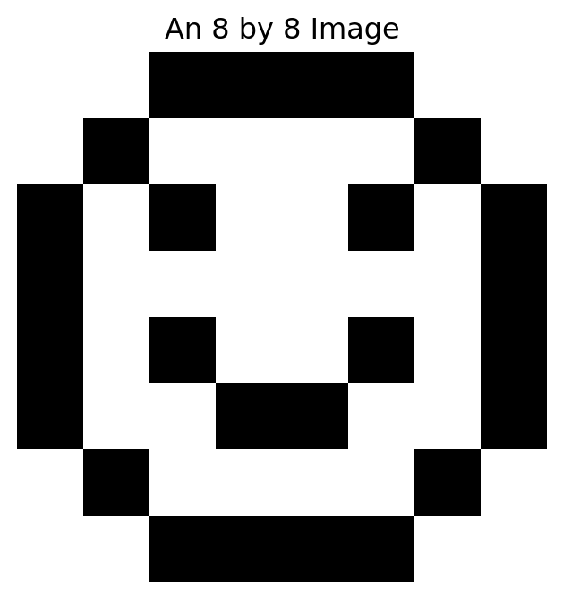
### Example: An Image as a Point
An $8 \times 8$ grayscale image can be flattened into a vector in $\mathbb{R}^{64}$.
```{python}
image = np.array([
    [0, 0, 1, 1, 1, 1, 0, 0],
    [0, 1, 0, 0, 0, 0, 1, 0],
    [1, 0, 1, 0, 0, 1, 0, 1],
    [1, 0, 0, 0, 0, 0, 0, 1],
    [1, 0, 1, 0, 0, 1, 0, 1],
    [1, 0, 0, 1, 1, 0, 0, 1],
    [0, 1, 0, 0, 0, 0, 1, 0],
    [0, 0, 1, 1, 1, 1, 0, 0]
])

plt.figure(figsize=(4, 4))
plt.imshow(image, cmap="gray_r")
plt.title("An 8 by 8 Image")
plt.axis("off")
plt.show()

image_vector = image.reshape(-1)
image_vector.shape
```
The image is a picture.
But it is also a point in $\mathbb{R}^{64}$.
This idea will return when we study images as matrices, SVD, compression, and neural networks.
## 4.9 Distance in Data Space
Once objects become points, we can compare them geometrically.
Suppose two students are represented by
$$
x=
\begin{bmatrix}
5 \\
85
\end{bmatrix},
\qquad
y=
\begin{bmatrix}
6 \\
88
\end{bmatrix}.
$$
Their difference is
$$
x-y=
\begin{bmatrix}
-1 \\
-3
\end{bmatrix}.
$$
Their Euclidean distance is
$$
\|x-y\|=\sqrt{(-1)^2+(-3)^2}=\sqrt{10}.
$$
A small distance suggests that the objects are similar with respect to the chosen features.
```{python}
x = np.array([5, 85])
y = np.array([6, 88])

np.linalg.norm(x - y)
```
::: {.callout-warning}
## Distance depends on representation
Distance is not an absolute truth.
It depends on which features we choose and how we scale them.
:::
## 4.10 Scaling Changes Geometry
Consider two houses:
$$
h_1=
\begin{bmatrix}
1800 \\
500000
\end{bmatrix},
\qquad
h_2=
\begin{bmatrix}
1900 \\
510000
\end{bmatrix},
$$
where the coordinates are square feet and price in dollars.
```{python}
h1 = np.array([1800, 500000])
h2 = np.array([1900, 510000])

np.linalg.norm(h1 - h2)
```
The price coordinate dominates the distance because it is measured in large units.
If price is measured in thousands of dollars, the vectors become
$$
\begin{bmatrix}
1800 \\
500
\end{bmatrix},
\qquad
\begin{bmatrix}
1900 \\
510
\end{bmatrix}.
$$
```{python}
h1_scaled = np.array([1800, 500])
h2_scaled = np.array([1900, 510])

np.linalg.norm(h1_scaled - h2_scaled)
```
The distance changed.
The houses did not change.
Only the representation changed.
This is a deep lesson:
> Changing units changes geometry.
### Standardization
A common scaling method is standardization.
For each feature, subtract its mean and divide by its standard deviation.
If a feature column is $x$, the standardized version is
$$
z=\frac{x-\bar{x}}{s},
$$
where $\bar{x}$ is the mean and $s$ is the standard deviation.
After standardization, each feature is measured in units of its own variability.
```{python}
H = np.array([
    [1400, 430000],
    [1800, 500000],
    [2100, 560000],
    [2500, 650000],
    [1600, 470000]
])

means = H.mean(axis=0)
stds = H.std(axis=0)
Z = (H - means) / stds

Z
```
Standardization does not solve every problem, but it often prevents one feature from dominating simply because of its units.
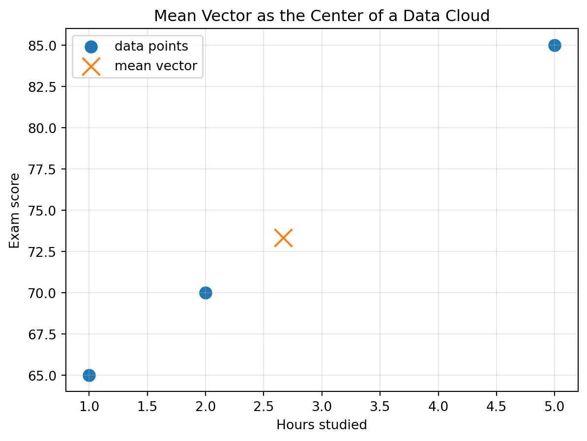
## 4.11 The Mean Vector: The Center of a Cloud
For a dataset of vectors, the mean vector is the average point.
If
$$
x_1, x_2, \ldots, x_m \in \mathbb{R}^n,
$$
then the mean vector is
$$
\bar{x}=\frac{1}{m}\sum_{i=1}^m x_i.
$$
For example,
$$
x_1=
\begin{bmatrix}
2 \\
70
\end{bmatrix},
\quad
x_2=
\begin{bmatrix}
5 \\
85
\end{bmatrix},
\quad
x_3=
\begin{bmatrix}
1 \\
65
\end{bmatrix}.
$$
Then
$$
\bar{x}=\frac{1}{3}
\left(
\begin{bmatrix}
2 \\
70
\end{bmatrix}
+
\begin{bmatrix}
5 \\
85
\end{bmatrix}
+
\begin{bmatrix}
1 \\
65
\end{bmatrix}
\right)
=
\begin{bmatrix}
8/3 \\
220/3
\end{bmatrix}.
$$
```{python}
X = np.array([
    [2, 70],
    [5, 85],
    [1, 65]
])

mean_vector = X.mean(axis=0)
mean_vector
```
```{python}
plt.figure(figsize=(7, 5))
plt.scatter(X[:, 0], X[:, 1], s=80, label="data points")
plt.scatter(mean_vector[0], mean_vector[1], s=180, marker="x", label="mean vector")
plt.xlabel("Hours studied")
plt.ylabel("Exam score")
plt.title("Mean Vector as the Center of a Data Cloud")
plt.legend()
plt.grid(True, alpha=0.3)
plt.show()
```
The mean vector is the center of the cloud.
It is not necessarily one of the observed points.
It is the balance point of the dataset.
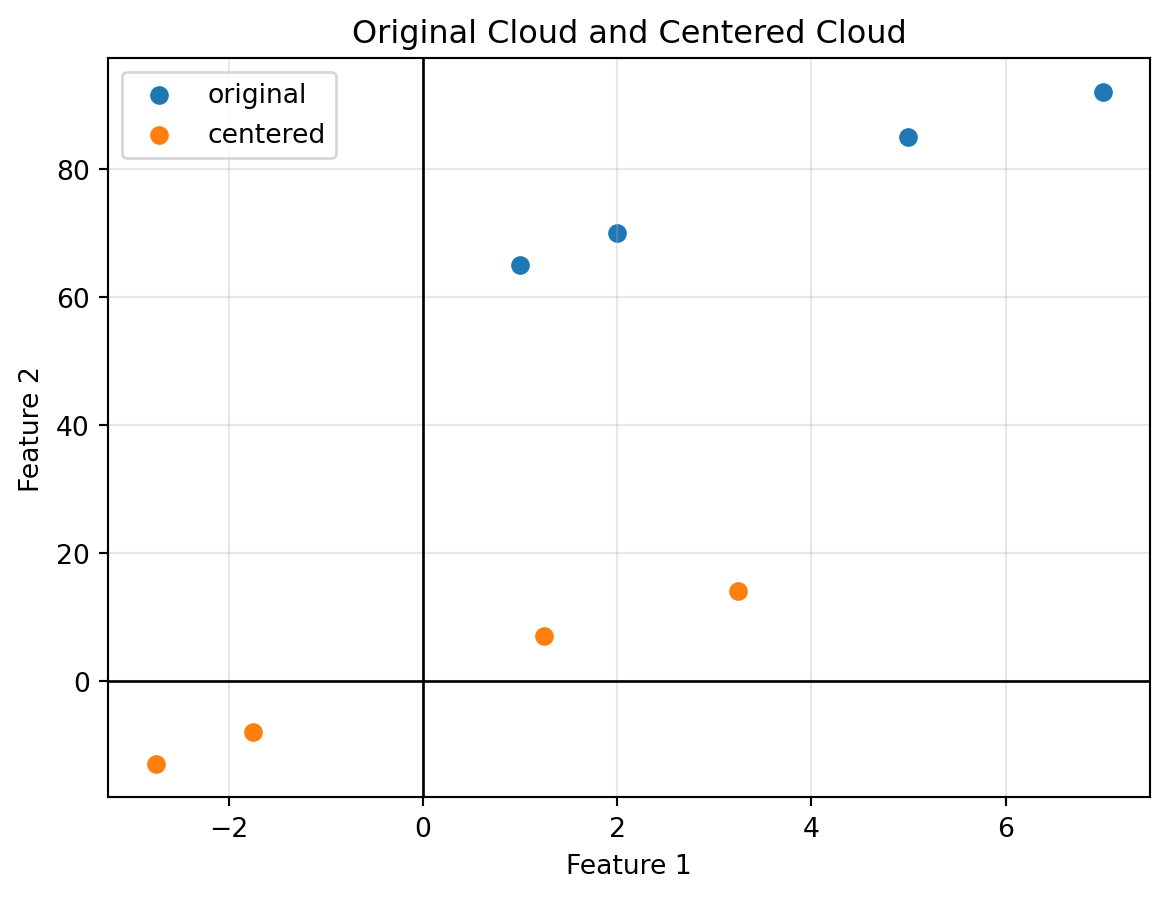
## 4.12 Centering Data
Centering means subtracting the mean vector from every data point.
If $x_i$ is a data point and $\bar{x}$ is the mean vector, then the centered point is
$$
x_i - \bar{x}.
$$
The centered dataset has mean zero.
```{python}
X = np.array([
    [2, 70],
    [5, 85],
    [1, 65],
    [7, 92]
])

X_centered = X - X.mean(axis=0)
X.mean(axis=0), X_centered, X_centered.mean(axis=0)
```
Centering moves the cloud so that its center is at the origin.
The shape of the cloud stays the same, but its location changes.
```{python}
plt.figure(figsize=(7, 5))
plt.scatter(X[:, 0], X[:, 1], label="original")
plt.scatter(X_centered[:, 0], X_centered[:, 1], label="centered")
plt.axhline(0, color="black", linewidth=1)
plt.axvline(0, color="black", linewidth=1)
plt.xlabel("Feature 1")
plt.ylabel("Feature 2")
plt.title("Original Cloud and Centered Cloud")
plt.legend()
plt.grid(True, alpha=0.3)
plt.show()
```
Centering is essential for many later tools, especially covariance, least squares, and PCA.
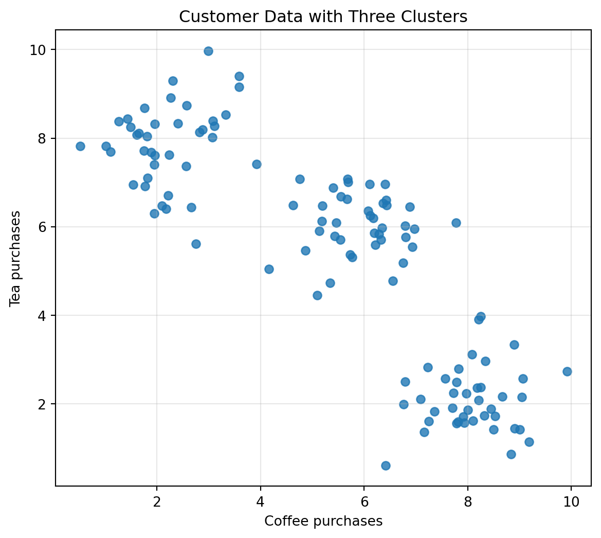
## 4.13 Clusters: Groups in the Cloud
Sometimes points form groups.
These groups are called clusters.
For example, suppose customers are described by two features:
$$
\begin{bmatrix}
\text{coffee purchases} \\
\text{tea purchases}
\end{bmatrix}.
$$
Some customers mostly buy coffee, some mostly buy tea, and some buy both.
```{python}
np.random.seed(10)
coffee = np.random.normal(loc=[8, 2], scale=[0.8, 0.8], size=(40, 2))
tea = np.random.normal(loc=[2, 8], scale=[0.8, 0.8], size=(40, 2))
both = np.random.normal(loc=[6, 6], scale=[0.8, 0.8], size=(40, 2))

C = np.vstack([coffee, tea, both])

plt.figure(figsize=(7, 6))
plt.scatter(C[:, 0], C[:, 1], alpha=0.8)
plt.xlabel("Coffee purchases")
plt.ylabel("Tea purchases")
plt.title("Customer Data with Three Clusters")
plt.grid(True, alpha=0.3)
plt.show()
```
A cluster suggests that some objects are more similar to one another than to the rest of the dataset.
Clustering is a major topic in machine learning, but its first idea is visual and geometric:
> Nearby points may belong together.
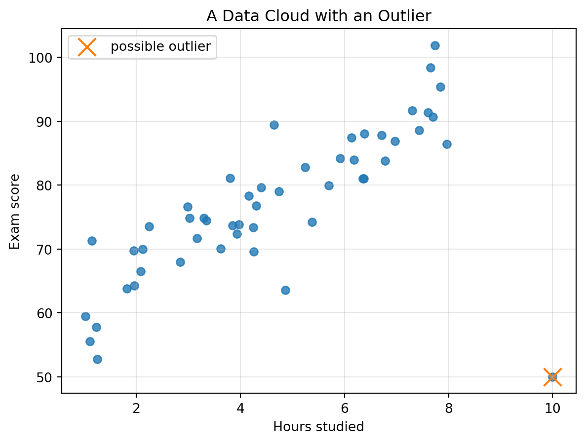
## 4.14 Outliers: Points That Refuse to Blend In
An outlier is a point far from the main cloud.
```{python}
np.random.seed(12)

hours = np.random.uniform(1, 8, 50)
scores = 55 + 5 * hours + np.random.normal(0, 5, size=50)

hours = np.append(hours, 10)
scores = np.append(scores, 50)

plt.figure(figsize=(7, 5))
plt.scatter(hours, scores, alpha=0.8)
plt.scatter([10], [50], s=180, marker="x", label="possible outlier")
plt.xlabel("Hours studied")
plt.ylabel("Exam score")
plt.title("A Data Cloud with an Outlier")
plt.legend()
plt.grid(True, alpha=0.3)
plt.show()
```
An outlier may be:
- a data entry error;
- an unusual but valid case;
- a special subgroup;
- a rare event;
- an important discovery.
::: {.callout-warning}
## Outliers require interpretation
An outlier is not automatically bad.
It is a point asking for an explanation.
:::
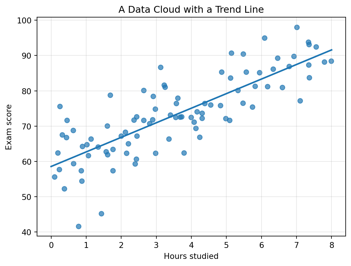
## 4.15 Trends and First Models
A trend is a general direction in a data cloud.
In the study-hours example, the cloud slopes upward. We can summarize the trend with a line.
```{python}
np.random.seed(15)

hours = np.random.uniform(0, 8, 90)
scores = 58 + 4.3 * hours + np.random.normal(0, 7, size=90)

m, b = np.polyfit(hours, scores, 1)
x_line = np.linspace(0, 8, 100)
y_line = m * x_line + b

plt.figure(figsize=(7, 5))
plt.scatter(hours, scores, alpha=0.7)
plt.plot(x_line, y_line, linewidth=2)
plt.xlabel("Hours studied")
plt.ylabel("Exam score")
plt.title("A Data Cloud with a Trend Line")
plt.grid(True, alpha=0.3)
plt.show()

m, b
```
This line is a simple model.
It compresses many points into a short rule:
$$
\text{predicted score} \approx m \cdot \text{hours} + b.
$$
Later, we will study least squares, where the central question is:
> Which line, plane, or higher-dimensional flat surface best fits the cloud?
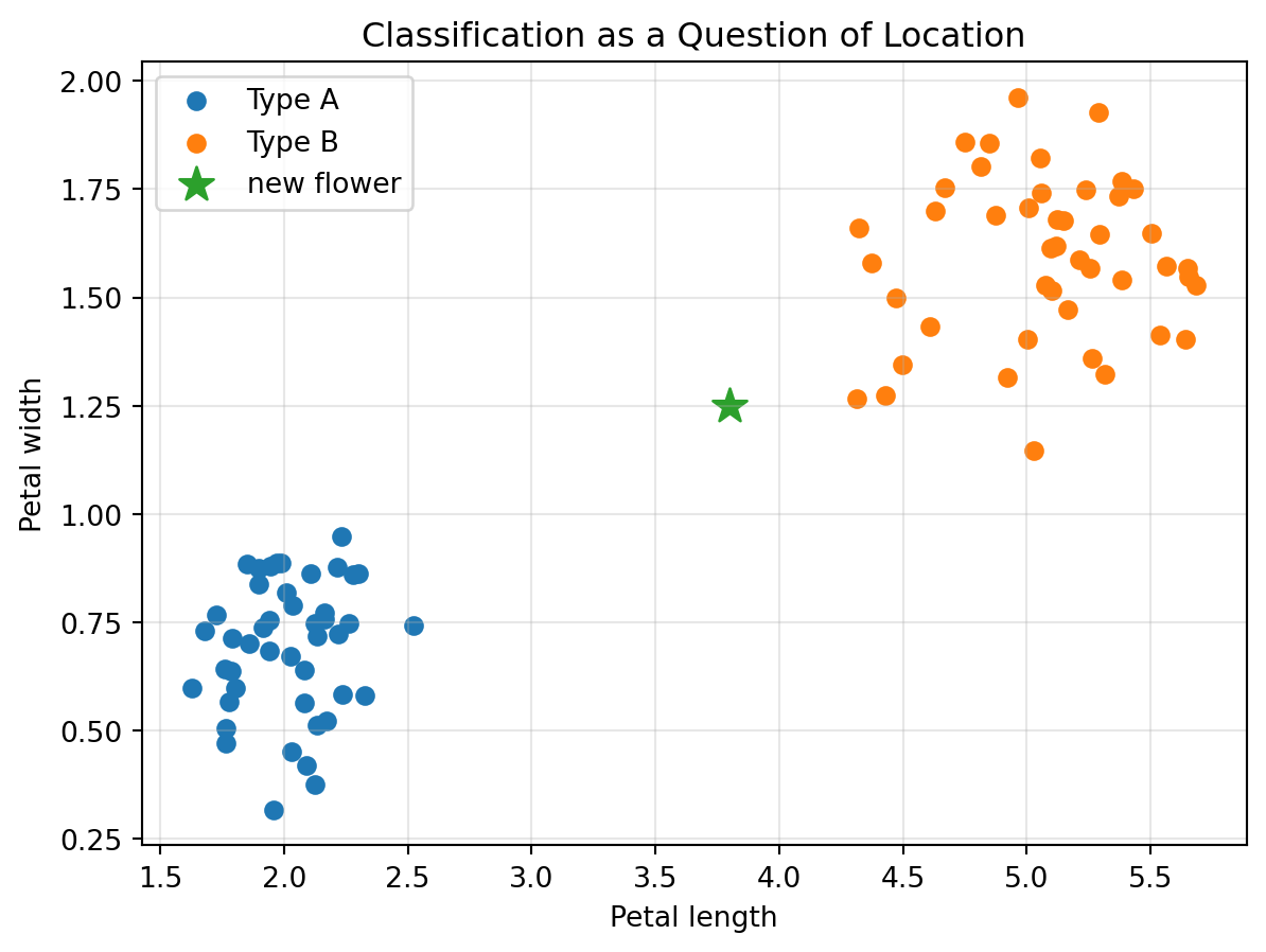
## 4.16 Classification Begins with Geometry
Suppose we measure flowers using two features:
$$
\begin{bmatrix}
\text{petal length} \\
\text{petal width}
\end{bmatrix}.
$$
Two flower types may produce two different clouds.
```{python}
np.random.seed(20)

type_A = np.random.normal(loc=[2.0, 0.7], scale=[0.25, 0.12], size=(45, 2))
type_B = np.random.normal(loc=[5.0, 1.6], scale=[0.35, 0.18], size=(45, 2))
new_flower = np.array([3.8, 1.25])

plt.figure(figsize=(7, 5))
plt.scatter(type_A[:, 0], type_A[:, 1], label="Type A")
plt.scatter(type_B[:, 0], type_B[:, 1], label="Type B")
plt.scatter(new_flower[0], new_flower[1], s=160, marker="*", label="new flower")
plt.xlabel("Petal length")
plt.ylabel("Petal width")
plt.title("Classification as a Question of Location")
plt.legend()
plt.grid(True, alpha=0.3)
plt.show()
```
A classification method asks:
> Where does the new point sit relative to known groups?
This does not solve all of classification, but it shows why geometry is the starting point.
## 4.17 Nearest Neighbors
One simple geometric idea is nearest-neighbor classification.
Given a new point, find the closest known points.
If most nearby points belong to one class, assign the new point to that class.
```{python}
X_train = np.vstack([type_A, type_B])
y_train = np.array([0] * len(type_A) + [1] * len(type_B))

distances = np.linalg.norm(X_train - new_flower, axis=1)
nearest_index = np.argmin(distances)
nearest_label = y_train[nearest_index]

nearest_index, nearest_label, distances[nearest_index]
```
This is not yet a full machine learning course.
But the core idea is clear:
> Classification can begin with distance in feature space.
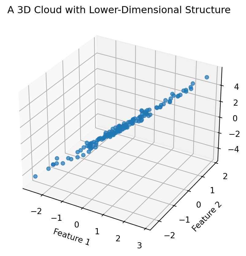
## 4.18 Dimension Reduction: Seeing a Shadow of a High-Dimensional Cloud
High-dimensional data is hard to visualize.
Dimension reduction means creating a lower-dimensional picture of a high-dimensional dataset while preserving important structure.
A simple way to reduce dimension is to keep only two features.
But a more powerful approach is to find a useful direction or plane.
For now, we can preview the idea with a three-dimensional cloud that mostly lies near a plane.
```{python}
np.random.seed(25)

t = np.random.normal(0, 1, 150)
u = np.random.normal(0, 0.5, 150)
noise = np.random.normal(0, 0.1, 150)

x = t
ny = 0.5 * t + u
z = 2 * t - u + noise
X3 = np.column_stack([x, ny, z])

fig = plt.figure(figsize=(7, 5))
ax = fig.add_subplot(111, projection="3d")
ax.scatter(X3[:, 0], X3[:, 1], X3[:, 2], alpha=0.7)
ax.set_xlabel("Feature 1")
ax.set_ylabel("Feature 2")
ax.set_zlabel("Feature 3")
ax.set_title("A 3D Cloud with Lower-Dimensional Structure")
plt.show()
```
The cloud lives in three dimensions, but it has a simpler shape.
Later, PCA will give us a systematic way to find such lower-dimensional structure.
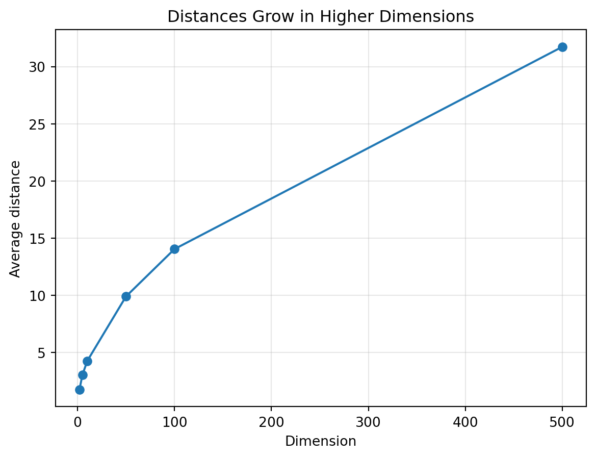
## 4.19 A First High-Dimensional Experiment
Let us create points in high-dimensional space and study their distances.
```{python}
np.random.seed(30)

dimensions = [2, 5, 10, 50, 100, 500]
mean_distances = []
std_distances = []

for d in dimensions:
    A = np.random.normal(size=(200, d))
    B = np.random.normal(size=(200, d))
    distances = np.linalg.norm(A - B, axis=1)
    mean_distances.append(distances.mean())
    std_distances.append(distances.std())

plt.figure(figsize=(7, 5))
plt.plot(dimensions, mean_distances, marker="o", label="mean distance")
plt.xlabel("Dimension")
plt.ylabel("Average distance")
plt.title("Distances Grow in Higher Dimensions")
plt.grid(True, alpha=0.3)
plt.show()
```
In high dimensions, geometry can behave differently from our two-dimensional intuition.
This is one reason modern data analysis needs careful mathematics.
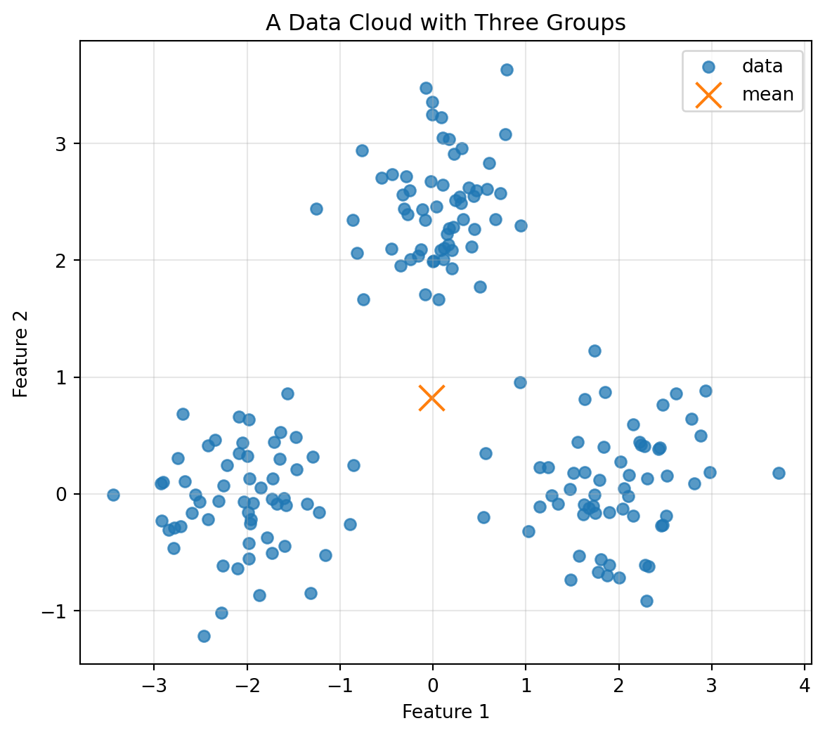
## 4.20 Mini-Lab: Build a Data Cloud from Scratch
In this mini-lab, we create a dataset with three groups and then analyze its center and spread.
```{python}
np.random.seed(40)

G1 = np.random.normal(loc=[-2, 0], scale=0.5, size=(60, 2))
G2 = np.random.normal(loc=[2, 0], scale=0.5, size=(60, 2))
G3 = np.random.normal(loc=[0, 2.5], scale=0.5, size=(60, 2))

X = np.vstack([G1, G2, G3])
mean = X.mean(axis=0)
X_centered = X - mean

plt.figure(figsize=(7, 6))
plt.scatter(X[:, 0], X[:, 1], alpha=0.75, label="data")
plt.scatter(mean[0], mean[1], s=180, marker="x", label="mean")
plt.xlabel("Feature 1")
plt.ylabel("Feature 2")
plt.title("A Data Cloud with Three Groups")
plt.legend()
plt.grid(True, alpha=0.3)
plt.show()
```
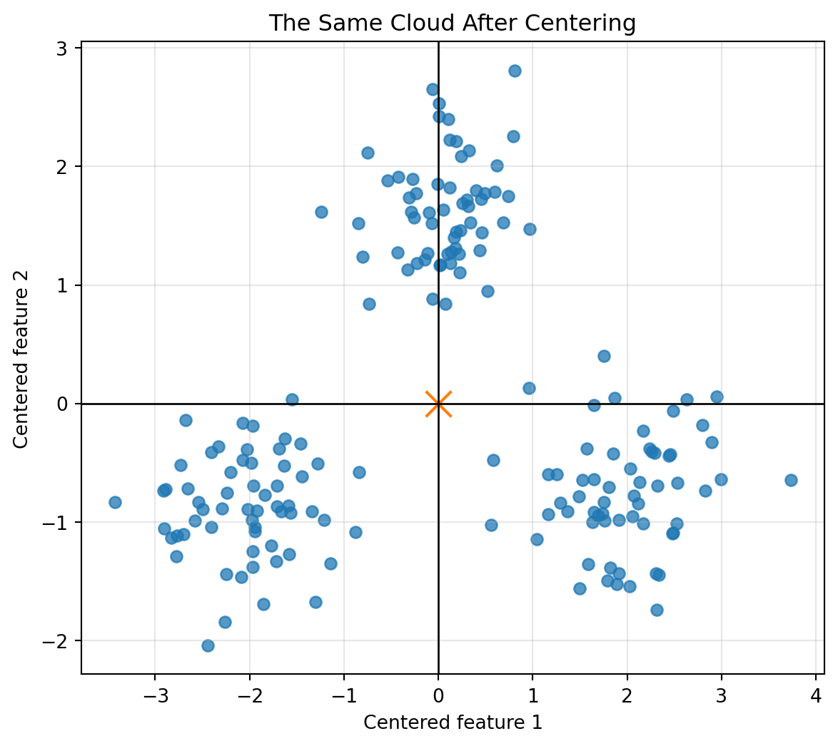
Now center the dataset.
```{python}
plt.figure(figsize=(7, 6))
plt.scatter(X_centered[:, 0], X_centered[:, 1], alpha=0.75)
plt.scatter(0, 0, s=180, marker="x")
plt.axhline(0, color="black", linewidth=1)
plt.axvline(0, color="black", linewidth=1)
plt.xlabel("Centered feature 1")
plt.ylabel("Centered feature 2")
plt.title("The Same Cloud After Centering")
plt.grid(True, alpha=0.3)
plt.show()
```
The cloud moved, but its shape did not change.
This is the basic idea behind centering: shift the origin to the center of the data.
## 4.21 Concept Summary
A dataset is a collection of vectors.
Each vector is a point in feature space.
A data matrix stores these vectors, usually with rows as objects and columns as features.
A data cloud is the geometric shape formed by many data points.
The shape of a data cloud may reveal trends, clusters, gaps, outliers, and hidden directions.
The mean vector is the center of the cloud.
Centering subtracts the mean vector from every point.
Scaling changes the geometry of the cloud because distance depends on units.
High-dimensional data is common because real objects often require many features.
The central message is:
> To understand data, learn to see the table as geometry.
## 4.22 Key Vocabulary
**Dataset**
A collection of objects or observations.
**Data point**
One object represented as a vector.
**Feature**
A coordinate used to describe an object.
**Feature space**
The coordinate space created by the selected features.
**Data cloud**
The collection of points formed by a dataset in feature space.
**Data matrix**
A matrix whose rows often represent objects and whose columns represent features.
**Row view**
The interpretation of each row of a data matrix as one object.
**Column view**
The interpretation of each column of a data matrix as one feature measured across objects.
**Mean vector**
The coordinate-wise average of the data points.
**Centering**
Subtracting the mean vector from every data point.
**Scaling**
Changing the numerical scale of features, often to make distances more meaningful.
**Cluster**
A group of nearby points.
**Outlier**
A point far from the main cloud or pattern.
**Trend**
A general direction or pattern in a data cloud.
**Dimension reduction**
Representing high-dimensional data in a lower-dimensional space while preserving important structure.
## 4.23 Practice Problems
### Problem 1
A student is represented by
$$
x=
\begin{bmatrix}
4 \\
7 \\
82
\end{bmatrix},
$$
where the coordinates are hours studied, sleep hours, and exam score.
Write a sentence interpreting this vector.
::: {.callout-tip collapse="true"}
## Solution
The vector describes a student who studied 4 hours, slept 7 hours, and earned an exam score of 82.
:::
### Problem 2
The following data matrix represents four students:
$$
X=
\begin{bmatrix}
2 & 7 & 70 \\
5 & 6 & 85 \\
1 & 8 & 65 \\
7 & 5 & 92
\end{bmatrix}.
$$
Answer:
1. How many students are represented?
2. How many features are measured?
3. What is the vector for the second student?
4. What is the feature vector for exam scores?
::: {.callout-tip collapse="true"}
## Solution
There are 4 students because there are 4 rows.
There are 3 features because there are 3 columns.
The second student is represented by
$$
\begin{bmatrix}
5 \\
6 \\
85
\end{bmatrix}.
$$
The exam score feature vector is
$$
\begin{bmatrix}
70 \\
85 \\
65 \\
92
\end{bmatrix}.
$$
:::
### Problem 3
Two restaurants are represented by
$$
r_1=
\begin{bmatrix}
2 \\
1 \\
4.5
\end{bmatrix},
\qquad
r_2=
\begin{bmatrix}
3 \\
2 \\
4.7
\end{bmatrix},
$$
where the coordinates are price level, distance in miles, and rating.
Compute $r_1-r_2$ and interpret it.
::: {.callout-tip collapse="true"}
## Solution
$$
r_1-r_2=
\begin{bmatrix}
2-3 \\
1-2 \\
4.5-4.7
\end{bmatrix}
=
\begin{bmatrix}
-1 \\
-1 \\
-0.2
\end{bmatrix}.
$$
Restaurant 1 is one price level lower, one mile closer, and has a rating 0.2 lower than Restaurant 2.
:::
### Problem 4
Give an example of a dataset where points might form clusters. What would the clusters mean?
::: {.callout-tip collapse="true"}
## Solution
A music dataset may contain songs described by tempo, energy, danceability, and acousticness. Clusters could correspond to musical styles such as dance music, acoustic songs, and slow ballads.
:::
### Problem 5
Give an example of an outlier in a real-world dataset. Would it be an error, an exception, or an important discovery?
::: {.callout-tip collapse="true"}
## Solution
In a dataset of daily website visits, one day may have ten times the usual number of visitors. It could be a tracking error, a special marketing event, or an important discovery about viral attention.
:::
### Problem 6
Why can changing units change distances between data points? Give an example.
::: {.callout-tip collapse="true"}
## Solution
Distance depends on coordinate values. If house price is measured in dollars, price differences may dominate size differences. If price is measured in thousands of dollars, the numerical scale changes, so the computed distances change.
:::
### Problem 7
Suppose
$$
X=
\begin{bmatrix}
1 & 2 \\
3 & 4 \\
5 & 6
\end{bmatrix}.
$$
Compute the mean vector and the centered matrix.
::: {.callout-tip collapse="true"}
## Solution
The mean vector is
$$
\bar{x}=\begin{bmatrix}3 & 4\end{bmatrix}.
$$
The centered matrix is
$$
X-\bar{x}=
\begin{bmatrix}
-2 & -2 \\
0 & 0 \\
2 & 2
\end{bmatrix}.
$$
:::
## 4.24 Python Practice
### Exercise 1: Create a Data Matrix
Create a data matrix with 6 objects and 4 features.
```{python}
X = np.array([
    [1.2, 3.4, 0.5, 10],
    [1.8, 3.1, 0.7, 12],
    [3.2, 1.5, 1.1, 18],
    [3.5, 1.2, 1.3, 20],
    [0.8, 4.0, 0.4, 9],
    [2.9, 1.8, 1.0, 17]
])

X.shape
```
### Exercise 2: Compute Feature Means
```{python}
X.mean(axis=0)
```
### Exercise 3: Center the Dataset
```{python}
X_centered = X - X.mean(axis=0)
X_centered.mean(axis=0)
```
### Exercise 4: Compare Distances Before and After Scaling
```{python}
a = np.array([1800, 500000])
b = np.array([1900, 510000])

raw_distance = np.linalg.norm(a - b)

A = np.array([
    [1800, 500000],
    [1900, 510000],
    [2500, 700000],
    [1200, 350000]
])
A_standardized = (A - A.mean(axis=0)) / A.std(axis=0)
scaled_distance = np.linalg.norm(A_standardized[0] - A_standardized[1])

raw_distance, scaled_distance
```
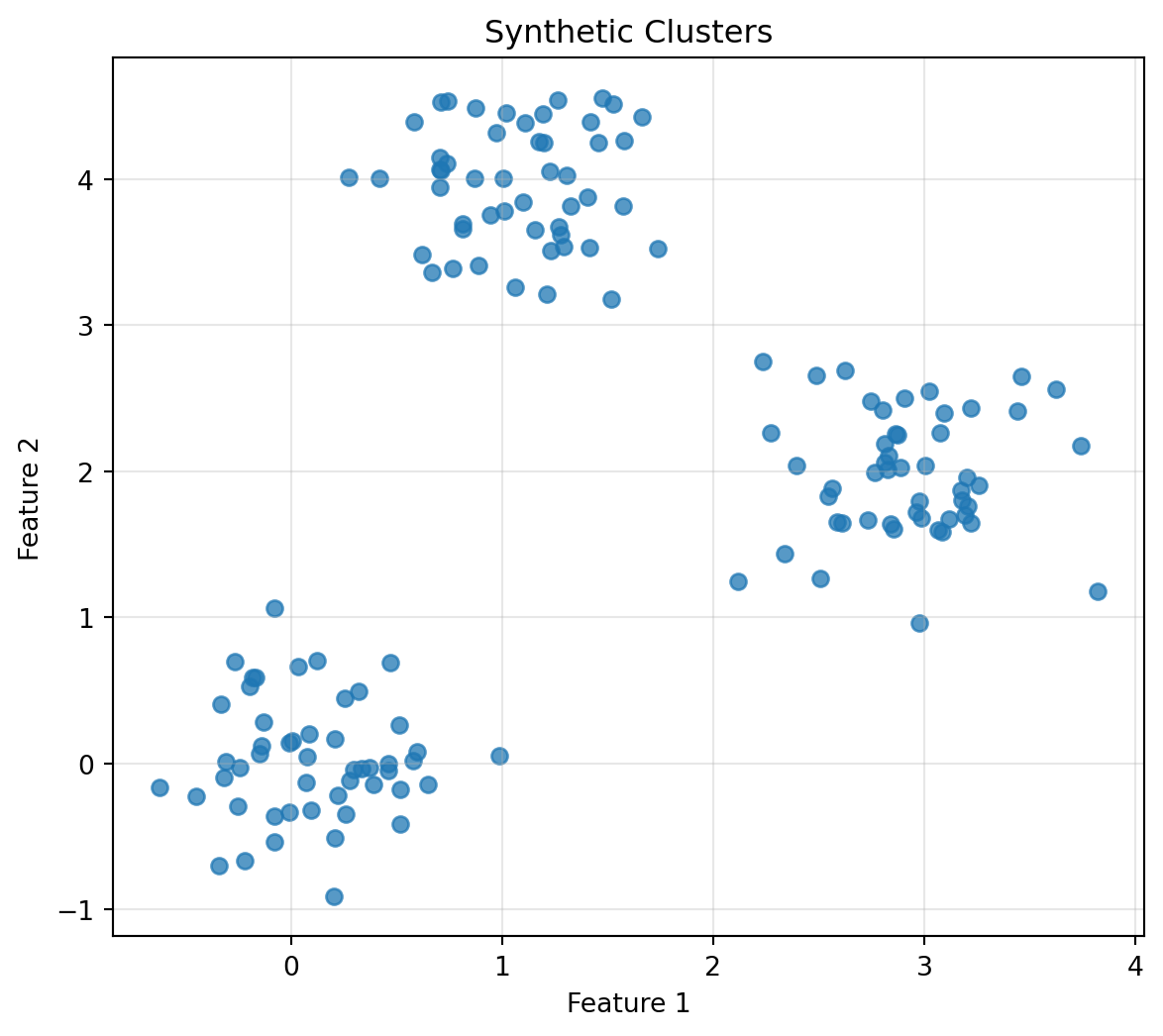
### Exercise 5: Generate and Plot Clusters
```{python}
np.random.seed(52)

cluster_1 = np.random.normal(loc=[0, 0], scale=0.4, size=(50, 2))
cluster_2 = np.random.normal(loc=[3, 2], scale=0.4, size=(50, 2))
cluster_3 = np.random.normal(loc=[1, 4], scale=0.4, size=(50, 2))

X_clusters = np.vstack([cluster_1, cluster_2, cluster_3])

plt.figure(figsize=(7, 6))
plt.scatter(X_clusters[:, 0], X_clusters[:, 1], alpha=0.75)
plt.xlabel("Feature 1")
plt.ylabel("Feature 2")
plt.title("Synthetic Clusters")
plt.grid(True, alpha=0.3)
plt.show()
```
### Exercise 6: High-Dimensional Data
Create 100 points in $\mathbb{R}^{50}$ and compute the mean vector.
```{python}
np.random.seed(60)

X_high = np.random.normal(size=(100, 50))
mean_high = X_high.mean(axis=0)

X_high.shape, mean_high.shape, np.linalg.norm(mean_high)
```
## 4.25 AI Companion Activities
### Activity 1: Explain the Big Idea
Ask an AI tool:
> Explain why a dataset can be viewed as a cloud of points in feature space. Use examples from students, houses, and images.
Then rewrite the explanation in your own words.
### Activity 2: Feature Design
Ask:
> Choose five useful features for representing restaurants as vectors. Explain how each feature affects distance between restaurants.
Then improve the feature list by removing one weak feature and adding one better feature.
### Activity 3: Scaling
Ask:
> Why does feature scaling matter when computing distance? Explain using houses described by size and price.
Then create your own example where one feature dominates the distance.
### Activity 4: Clusters and Outliers
Ask:
> Give three examples where clusters are useful and three examples where outliers are important discoveries.
Then decide which examples are classification problems, clustering problems, or anomaly detection problems.
### Activity 5: High-Dimensional Thinking
Ask:
> Explain high-dimensional data to a beginner using images, text documents, and recommendation systems.
Then write a short paragraph beginning with: "High-dimensional data is not mysterious because..."
## 4.26 Reflection Questions
1. Why does a dataset become a cloud of points?
2. What is feature space?
3. How does the choice of features affect the geometry of data?
4. What is the difference between the row view and the column view of a data matrix?
5. What does a cluster suggest?
6. Why should outliers be interpreted carefully?
7. Why is high-dimensional data common?
8. Why can scaling change nearest neighbors?
9. What does the mean vector represent?
10. Why is centering useful?
11. How does this chapter prepare us for PCA and machine learning?
## 4.27 Chapter Closing
In this chapter, a table became a shape.
A row became a point.
A collection of rows became a cloud.
The cloud could stretch, split into clusters, hide outliers, or point in a direction.
This is the beginning of the geometric view of data.
When we look at a dataset through linear algebra, we do not only ask:
> What numbers are in the table?
We also ask:
> What shape do these numbers make?
In the next chapter, we introduce matrices as machines.
A matrix does not merely store a dataset.
A matrix can transform vectors, move clouds, mix features, compress information, and become the engine of algorithms.