import numpy as np
import matplotlib.pyplot as plt26 Python Reference for Computational Linear Algebra
This appendix is a practical Python reference for Computational Linear Algebra in \(\\mathbb{R}^n\).
It collects the most useful commands, patterns, and examples used throughout the book. The goal is not to teach all of Python. The goal is to help you use Python effectively for vectors, matrices, geometry, algorithms, and data.
The main packages are:
numpyfor arrays and numerical linear algebra,matplotlibfor plots and visualizations,sympyfor exact symbolic computations,- occasionally
pandasfor tabular data.
26.1 1. Basic setup
Most chapters begin with:
For exact symbolic computation, use:
import sympy as spFor data tables, use:
import pandas as pd26.2 2. NumPy arrays
A vector is represented by a one-dimensional NumPy array.
x = np.array([1, 2, 3], dtype=float)
x
array([1., 2., 3.])A matrix is represented by a two-dimensional NumPy array.
A = np.array([
    [1, 2, 3],
    [4, 5, 6]
], dtype=float)

A
array([[1., 2., 3.],
[4., 5., 6.]])The option dtype=float is often useful because linear algebra computations usually use real numbers.
26.3 3. Shapes and dimensions
Use .shape to check dimensions.
A.shape(2, 3)For a vector:
x.shape(3,)For a matrix \(A\in\mathbb{R}^{m\times n}\), A.shape returns:
(m, n)Dimension checking is essential. Many errors in linear algebra code come from incompatible matrix sizes.
26.4 4. Row vectors, column vectors, and one-dimensional arrays
In NumPy, a vector like
x = np.array([1, 2, 3], dtype=float)
x.shape(3,)has shape (3,), not (3, 1).
To create an explicit column vector:
x_col = np.array([[1],
                  [2],
                  [3]], dtype=float)

x_col.shape
(3, 1)To reshape a one-dimensional array into a column vector:
x = np.array([1, 2, 3], dtype=float)
x_col = x.reshape(-1, 1)

x_col
array([[1.],
[2.],
[3.]])To reshape into a row vector:
x_row = x.reshape(1, -1)
x_row
array([[1., 2., 3.]])26.5 5. Matrix and vector arithmetic
26.5.1 Addition
A = np.array([[1, 2],
              [3, 4]], dtype=float)

B = np.array([[5, 6],
              [7, 8]], dtype=float)

A + B
array([[ 6., 8.],
[10., 12.]])26.5.2 Scalar multiplication
3 * Aarray([[ 3., 6.],
[ 9., 12.]])26.5.3 Entrywise multiplication
A * Barray([[ 5., 12.],
[21., 32.]])This is not matrix multiplication. It multiplies corresponding entries.
26.5.4 Matrix multiplication
Use @ for matrix multiplication.
A @ Barray([[19., 22.],
[43., 50.]])Matrix-vector multiplication:
x = np.array([1, 2], dtype=float)

A @ x
array([ 5., 11.])26.6 6. Transpose
Use .T.
A.Tarray([[1., 3.],
[2., 4.]])Transpose changes rows into columns and columns into rows.
If \(A\) is \(m\times n\), then \(A^T\) is \(n\times m\).
26.7 7. Identity, zero, and diagonal matrices
26.7.1 Identity matrix
I = np.eye(3)
I
array([[1., 0., 0.],
[0., 1., 0.],
[0., 0., 1.]])26.7.2 Zero matrix
Z = np.zeros((3, 4))
Z
array([[0., 0., 0., 0.],
[0., 0., 0., 0.],
[0., 0., 0., 0.]])26.7.3 Ones matrix
O = np.ones((2, 3))
O
array([[1., 1., 1.],
[1., 1., 1.]])26.7.4 Diagonal matrix
D = np.diag([4, 2, -1])
D
array([[ 4, 0, 0],
[ 0, 2, 0],
[ 0, 0, -1]])26.7.5 Extract diagonal entries
np.diag(D)array([ 4, 2, -1])26.8 8. Building matrices from columns
Suppose we have column vectors:
v1 = np.array([1, 2, 3], dtype=float)
v2 = np.array([4, 5, 6], dtype=float)
v3 = np.array([7, 8, 9], dtype=float)
Build a matrix with these as columns:
A = np.column_stack([v1, v2, v3])
A
array([[1., 4., 7.],
[2., 5., 8.],
[3., 6., 9.]])Build a matrix with these as rows:
B = np.vstack([v1, v2, v3])
B
array([[1., 2., 3.],
[4., 5., 6.],
[7., 8., 9.]])26.9 9. Accessing entries, rows, and columns
A = np.array([
    [1, 2, 3],
    [4, 5, 6],
    [7, 8, 9]
], dtype=float)
Entry in row 0, column 1:
A[0, 1]2.0First row:
A[0, :]array([1., 2., 3.])Second column:
A[:, 1]array([2., 5., 8.])Top-left \(2\times 2\) block:
A[:2, :2]array([[1., 2.],
[4., 5.]])Remember that Python uses zero-based indexing.
26.10 10. Dot products, norms, and distances
26.10.1 Dot product
x = np.array([1, 2, 3], dtype=float)
y = np.array([4, 5, 6], dtype=float)

np.dot(x, y)32.0Equivalently:
x @ y32.026.10.2 Norm
np.linalg.norm(x)3.7416573867739413This computes the Euclidean norm:
\[ \|x\|=\sqrt{x_1^2+\cdots+x_n^2}. \]
26.10.3 Distance
np.linalg.norm(x - y)5.19615242270663226.10.4 Cosine similarity
def cosine_similarity(x, y):
    return np.dot(x, y) / (np.linalg.norm(x) * np.linalg.norm(y))

cosine_similarity(x, y)0.974631846197076226.11 11. Solving linear systems
To solve
\[ Ax=b, \]
use np.linalg.solve when \(A\) is square and invertible.
A = np.array([[2, 1],
              [1, 3]], dtype=float)

b = np.array([1, 2], dtype=float)

x = np.linalg.solve(A, b)
x
array([0.2, 0.6])Check the solution:
A @ xarray([1., 2.])26.11.1 Do not use the inverse unnecessarily
This works:
np.linalg.inv(A) @ barray([0.2, 0.6])But for solving systems, this is preferred:
np.linalg.solve(A, b)It is usually faster and more stable.
26.12 12. Row reduction with SymPy
NumPy is numerical. SymPy can compute exact reduced row echelon form.
M = sp.Matrix([
    [1, 2, 1, 4],
    [2, 4, 0, 6],
    [1, 1, 1, 3]
])

rref_M, pivots = M.rref()

rref_M, pivots
(Matrix([
[1, 0, 0, 1],
[0, 1, 0, 1],
[0, 0, 1, 1]]),
(0, 1, 2))The variable pivots gives the pivot columns.
26.13 13. Rank
Numerical rank:
A = np.array([
    [1, 2, 3],
    [2, 4, 6],
    [1, 1, 1]
], dtype=float)

np.linalg.matrix_rank(A)2Exact rank with SymPy:
sp.Matrix(A).rank()2Rank is the number of independent columns, the number of pivot columns, and the dimension of the column space.
26.14 14. Inverses
A = np.array([[2, 1],
              [1, 3]], dtype=float)

A_inv = np.linalg.inv(A)
A_inv
array([[ 0.6, -0.2],
[-0.2, 0.4]])Check:
A @ A_invarray([[ 1.00000000e+00, 0.00000000e+00],
[-5.55111512e-17, 1.00000000e+00]])Because of numerical roundoff, the result may be very close to the identity rather than exactly equal.
Use:
np.allclose(A @ A_inv, np.eye(2))True26.15 15. Determinants
A = np.array([[2, 1],
              [1, 3]], dtype=float)

np.linalg.det(A)5.000000000000001For exact determinants:
sp.Matrix([[2, 1],
           [1, 3]]).det()
\(\displaystyle 5\)
A square matrix is invertible if and only if its determinant is nonzero.
Numerically, use caution: a determinant close to zero suggests the matrix may be ill-conditioned.
26.16 16. Column space and null space with SymPy
SymPy can compute exact bases.
A = sp.Matrix([
    [1, 2, 3],
    [2, 4, 6],
    [1, 1, 1]
])

A.columnspace()
[Matrix([
[1],
[2],
[1]]),
Matrix([
[2],
[4],
[1]])]Null space:
A.nullspace()[Matrix([
[ 1],
[-2],
[ 1]])]Row space:
A.rowspace()[Matrix([[1, 2, 3]]), Matrix([[0, -1, -2]])]26.17 17. Linear combinations and span
Suppose the columns of \(A\) are vectors \(v_1,\ldots,v_n\).
To check whether \(b\) is in their span, solve
\[ Ax=b. \]
A = np.array([[1, 3],
              [2, 1]], dtype=float)

b = np.array([4, 3], dtype=float)

x = np.linalg.solve(A, b)
x
array([1., 1.])Then
A @ xarray([4., 3.])If a solution exists, then \(b\) lies in the span of the columns of \(A\).
For non-square or rank-deficient systems, use SymPy row reduction or least squares depending on the question.
26.18 18. Least squares
For an inconsistent or overdetermined system
\[ Ax\approx b, \]
use:
A = np.array([
    [1, 0],
    [1, 1],
    [1, 2],
    [1, 3]
], dtype=float)

b = np.array([1, 2, 2, 4], dtype=float)

x_hat, residuals, rank, singular_values = np.linalg.lstsq(A, b, rcond=None)

x_hat
array([0.9, 0.9])Predicted values:
b_hat = A @ x_hat
b_hat
array([0.9, 1.8, 2.7, 3.6])Residual:
r = b - b_hat
r
array([ 0.1, 0.2, -0.7, 0.4])Check orthogonality of residual to column space:
A.T @ rarray([-3.33066907e-16, -6.66133815e-16])This should be close to zero.
26.19 19. Linear regression
A line has form
\[ y=\beta_0+\beta_1t. \]
Build the design matrix with a column of ones:
t = np.array([0, 1, 2, 3], dtype=float)
y = np.array([1, 2, 2, 4], dtype=float)

A = np.column_stack([np.ones_like(t), t])

beta = np.linalg.lstsq(A, y, rcond=None)[0]
beta
array([0.9, 0.9])Predictions:
y_hat = A @ beta
y_hat
array([0.9, 1.8, 2.7, 3.6])Plot:
plt.figure(figsize=(6, 4))
plt.scatter(t, y, label="data")
plt.plot(t, y_hat, label="least-squares line")
plt.xlabel("$t$")
plt.ylabel("$y$")
plt.grid(True)
plt.legend()
plt.title("Linear regression")
plt.show()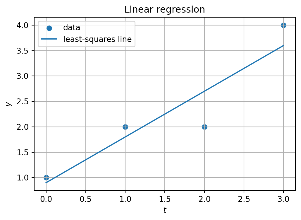
26.20 20. Polynomial regression
A quadratic model has form
\[ y=\beta_0+\beta_1t+\beta_2t^2. \]
t = np.linspace(-3, 3, 40)
rng = np.random.default_rng(0)

y = 1 - 0.5*t + 0.8*t**2 + rng.normal(scale=1.0, size=len(t))

A = np.column_stack([np.ones_like(t), t, t**2])

beta = np.linalg.lstsq(A, y, rcond=None)[0]

t_grid = np.linspace(-3.2, 3.2, 200)
A_grid = np.column_stack([np.ones_like(t_grid), t_grid, t_grid**2])
y_fit = A_grid @ beta

plt.figure(figsize=(6, 4))
plt.scatter(t, y, s=18, label="data")
plt.plot(t_grid, y_fit, label="quadratic fit")
plt.xlabel("$t$")
plt.ylabel("$y$")
plt.grid(True)
plt.legend()
plt.title("Polynomial regression")
plt.show()

beta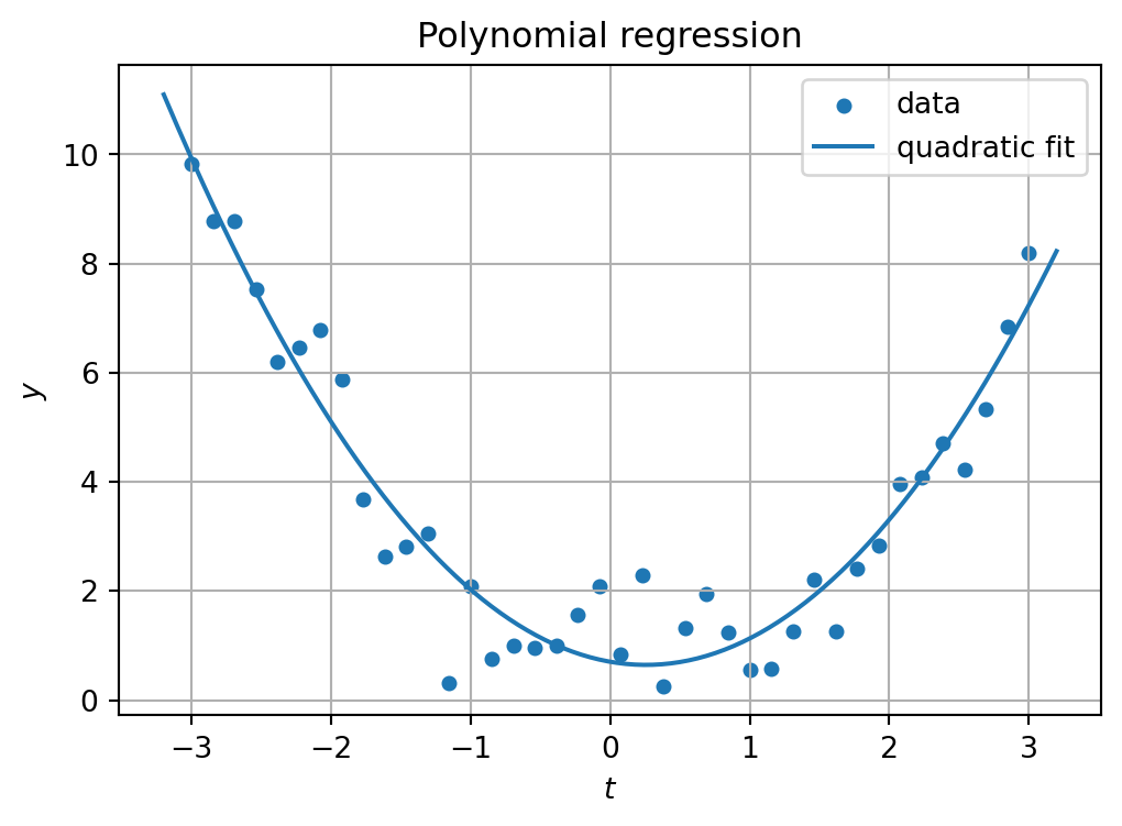
array([ 0.70267515, -0.44845021, 0.87510847])26.21 21. Orthogonal projection onto a line
Projection of \(b\) onto the line spanned by \(a\):
\[ \operatorname{proj}_{a}(b)=\frac{a\cdot b}{a\cdot a}a. \]
a = np.array([2, 1], dtype=float)
b = np.array([1, 3], dtype=float)

p = (np.dot(a, b) / np.dot(a, a)) * a
p
array([2., 1.])Residual:
e = b - p
np.dot(e, a)0.0The dot product should be zero.
26.22 22. Projection matrix onto a line
a = np.array([2, 1], dtype=float).reshape(-1, 1)

P = (a @ a.T) / (a.T @ a)

P
array([[0.8, 0.4],
[0.4, 0.2]])Project \(b\):
b = np.array([1, 3], dtype=float)

p = P @ b
p
array([2., 1.])Check projection matrix properties:
np.allclose(P @ P, P), np.allclose(P.T, P)(True, True)26.23 23. Projection onto a column space
If \(A\) has independent columns, the projection matrix onto \(\operatorname{Col}(A)\) is
\[ P=A(A^TA)^{-1}A^T. \]
A = np.array([
    [1, 0],
    [1, 1],
    [1, 2]
], dtype=float)

P = A @ np.linalg.inv(A.T @ A) @ A.T

P
array([[ 0.83333333, 0.33333333, -0.16666667],
[ 0.33333333, 0.33333333, 0.33333333],
[-0.16666667, 0.33333333, 0.83333333]])Project a vector:
b = np.array([1, 2, 4], dtype=float)

b_hat = P @ b
b_hat
array([0.83333333, 2.33333333, 3.83333333])Residual orthogonality:
r = b - b_hat
A.T @ r
array([1.11022302e-15, 8.88178420e-16])26.24 24. QR factorization
A = np.array([
    [1, 0],
    [1, 1],
    [1, 2]
], dtype=float)

Q, R = np.linalg.qr(A, mode="reduced")

Q, R
(array([[-5.77350269e-01, 7.07106781e-01],
[-5.77350269e-01, 4.43378006e-17],
[-5.77350269e-01, -7.07106781e-01]]),
array([[-1.73205081, -1.73205081],
[ 0. , -1.41421356]]))Check:
np.allclose(A, Q @ R)TrueCheck orthonormal columns:
Q.T @ Qarray([[1.00000000e+00, 3.39032612e-18],
[3.39032612e-18, 1.00000000e+00]])26.24.1 Least squares with QR
If
\[ A=QR, \]
then solve
\[ R\hat x=Q^Tb. \]
b = np.array([1, 2, 4], dtype=float)

x_hat = np.linalg.solve(R, Q.T @ b)
x_hat
array([0.83333333, 1.5 ])Compare:
np.linalg.lstsq(A, b, rcond=None)[0]array([0.83333333, 1.5 ])26.25 25. Eigenvalues and eigenvectors
For a square matrix:
A = np.array([[2, 1],
              [1, 2]], dtype=float)

eigvals, eigvecs = np.linalg.eig(A)

eigvals, eigvecs
(array([3., 1.]),
array([[ 0.70710678, -0.70710678],
[ 0.70710678, 0.70710678]]))Columns of eigvecs are eigenvectors.
Check:
for j in range(len(eigvals)):
    lam = eigvals[j]
    v = eigvecs[:, j]
    print("lambda =", lam)
    print("A v =", A @ v)
    print("lambda v =", lam * v)
    print()
lambda = 3.0
A v = [2.12132034 2.12132034]
lambda v = [2.12132034 2.12132034]
lambda = 1.0
A v = [-0.70710678 0.70710678]
lambda v = [-0.70710678 0.70710678]
26.26 26. Symmetric eigenvalue problems
For symmetric matrices, use np.linalg.eigh.
A = np.array([[2, 1],
              [1, 2]], dtype=float)

eigvals, Q = np.linalg.eigh(A)

eigvals, Q
(array([1., 3.]),
array([[-0.70710678, 0.70710678],
[ 0.70710678, 0.70710678]]))Check orthonormality:
Q.T @ Qarray([[1.00000000e+00, 2.23711432e-17],
[2.23711432e-17, 1.00000000e+00]])Check diagonalization:
D = np.diag(eigvals)

Q.T @ A @ Q, D
(array([[ 1.00000000e+00, 2.23711432e-17],
[-4.39088730e-17, 3.00000000e+00]]),
array([[1., 0.],
[0., 3.]]))Reconstruction:
Q @ D @ Q.Tarray([[2., 1.],
[1., 2.]])26.27 27. Diagonalization
If \(A=PDP^{-1}\), then:
A = np.array([[2, 1],
              [1, 2]], dtype=float)

eigvals, P = np.linalg.eig(A)
D = np.diag(eigvals)

A_reconstructed = P @ D @ np.linalg.inv(P)

A_reconstructed
array([[2., 1.],
[1., 2.]])Check:
np.allclose(A, A_reconstructed)TrueMatrix powers by diagonalization:
k = 5
A_power = P @ np.linalg.matrix_power(D, k) @ np.linalg.inv(P)

A_power
array([[122., 121.],
[121., 122.]])Compare:
np.linalg.matrix_power(A, k)array([[122., 121.],
[121., 122.]])26.28 28. Discrete dynamical systems
For
\[ x_{k+1}=Ax_k, \]
simulate by repeated multiplication.
A = np.array([[0.8, 0.1],
              [0.2, 0.7]], dtype=float)

x = np.array([1.0, 0.0])

history = [x.copy()]

for k in range(20):
    x = A @ x
    history.append(x.copy())

history = np.array(history)

history[:5]
array([[1. , 0. ],
[0.8 , 0.2 ],
[0.66 , 0.3 ],
[0.558 , 0.342 ],
[0.4806, 0.351 ]])Plot components:
plt.figure(figsize=(6, 4))
plt.plot(history[:, 0], marker="o", label="$x_1$")
plt.plot(history[:, 1], marker="o", label="$x_2$")
plt.xlabel("step")
plt.ylabel("value")
plt.grid(True)
plt.legend()
plt.title("Discrete dynamical system")
plt.show()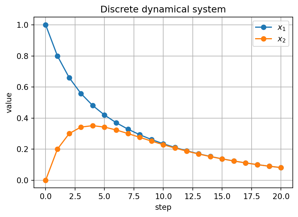
26.29 29. Singular value decomposition
For any matrix:
A = np.array([
    [2, 1],
    [0, 1],
    [1, 0]
], dtype=float)

U, s, Vt = np.linalg.svd(A, full_matrices=False)

U, s, Vt
(array([[-9.12870929e-01, -1.02407944e-16],
[-1.82574186e-01, -8.94427191e-01],
[-3.65148372e-01, 4.47213595e-01]]),
array([2.44948974, 1. ]),
array([[-0.89442719, -0.4472136 ],
[ 0.4472136 , -0.89442719]]))Reconstruct:
A_reconstructed = (U * s) @ Vt

A_reconstructed
array([[ 2.00000000e+00, 1.00000000e+00],
[-1.17756758e-16, 1.00000000e+00],
[ 1.00000000e+00, -1.67407441e-16]])Check:
np.allclose(A, A_reconstructed)TrueThe vector s contains singular values.
26.30 30. Rank from singular values
s = np.linalg.svd(A, compute_uv=False)
s
array([2.44948974, 1. ])Rank:
np.linalg.matrix_rank(A)2Numerical rank can be estimated by counting singular values above a tolerance.
tol = 1e-10
np.sum(s > tol)226.31 31. Condition number
A = np.array([[1, 0],
              [0, 0.001]], dtype=float)

np.linalg.cond(A)1000.0A large condition number means the matrix is close to singular or strongly stretches different directions by very different amounts.
26.32 32. Low-rank approximation
Use truncated SVD.
rng = np.random.default_rng(1)

m, n = 50, 40

X_true = (
    3 * np.outer(rng.normal(size=m), rng.normal(size=n))
    + 1.5 * np.outer(rng.normal(size=m), rng.normal(size=n))
)

X_noisy = X_true + 0.5 * rng.normal(size=(m, n))

U, s, Vt = np.linalg.svd(X_noisy, full_matrices=False)

def rank_k_approx(U, s, Vt, k):
    return (U[:, :k] * s[:k]) @ Vt[:k, :]

X_rank2 = rank_k_approx(U, s, Vt, 2)

np.linalg.norm(X_noisy - X_true), np.linalg.norm(X_rank2 - X_true)
(22.685934172734683, 6.674531107339763)26.33 33. Plotting singular values
plt.figure(figsize=(6, 4))
plt.plot(np.arange(1, len(s) + 1), s, marker="o")
plt.xlabel("index")
plt.ylabel("singular value")
plt.grid(True)
plt.title("Singular values")
plt.show()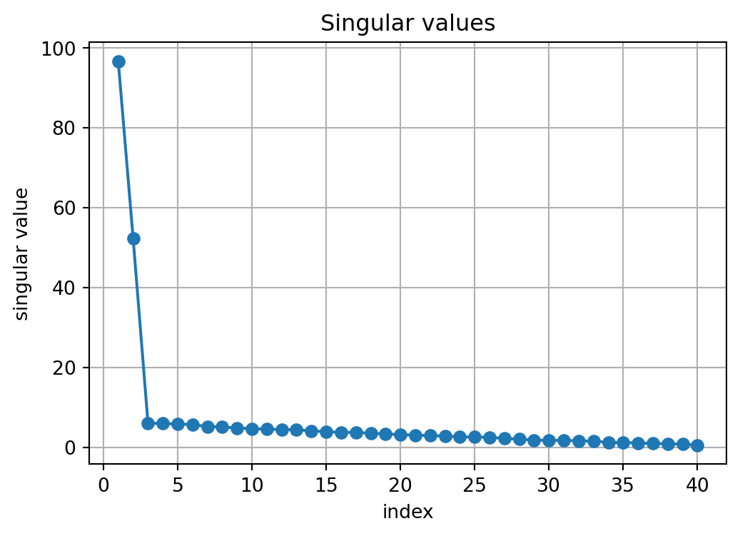
Cumulative energy:
energy = np.cumsum(s**2) / np.sum(s**2)

plt.figure(figsize=(6, 4))
plt.plot(np.arange(1, len(energy) + 1), energy, marker="o")
plt.xlabel("rank k")
plt.ylabel("cumulative energy")
plt.ylim(0, 1.05)
plt.grid(True)
plt.title("Cumulative energy")
plt.show()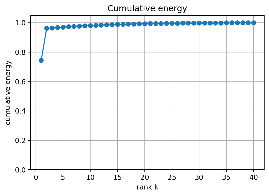
26.34 34. Pseudoinverse
A = np.array([
    [1, 2],
    [2, 4],
    [3, 6]
], dtype=float)

b = np.array([1, 2, 2], dtype=float)

x_pinv = np.linalg.pinv(A) @ b
x_pinv
array([0.15714286, 0.31428571])Compare with least squares:
np.linalg.lstsq(A, b, rcond=None)[0]array([0.15714286, 0.31428571])The pseudoinverse gives the minimum-norm least-squares solution.
26.35 35. PCA with SVD
Suppose rows are observations and columns are features.
rng = np.random.default_rng(2)

X = rng.multivariate_normal(
    mean=[3, 5],
    cov=[[4, 1.5], [1.5, 1]],
    size=300
)

Xc = X - X.mean(axis=0)

U, s, Vt = np.linalg.svd(Xc, full_matrices=False)

principal_directions = Vt.T
explained_variance = s**2 / (len(Xc) - 1)

principal_directions, explained_variance
(array([[ 0.92894786, -0.37021057],
[ 0.37021057, 0.92894786]]),
array([4.53113653, 0.38175544]))Plot data and principal directions:
plt.figure(figsize=(6, 6))
plt.scatter(Xc[:, 0], Xc[:, 1], s=12, alpha=0.5)

for j in range(2):
    direction = principal_directions[:, j]
    length = np.sqrt(explained_variance[j])
    plt.arrow(0, 0, length * direction[0], length * direction[1],
              head_width=0.08, length_includes_head=True)
    plt.text(length * direction[0], length * direction[1], f"$v_{j+1}$")

plt.axhline(0, linewidth=0.8)
plt.axvline(0, linewidth=0.8)
plt.grid(True)
plt.axis("equal")
plt.title("PCA by SVD")
plt.show()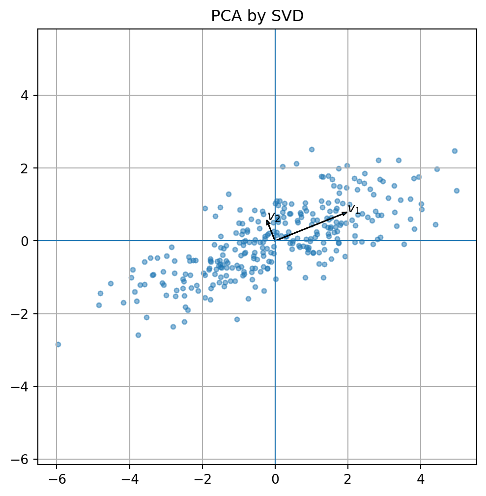
26.36 36. Projection onto principal components
Project onto the first principal direction:
V1 = principal_directions[:, :1]

Z = Xc @ V1
Xc_hat = Z @ V1.T

plt.figure(figsize=(6, 6))
plt.scatter(Xc[:, 0], Xc[:, 1], s=12, alpha=0.35, label="centered data")
plt.scatter(Xc_hat[:, 0], Xc_hat[:, 1], s=12, alpha=0.7, label="rank-1 reconstruction")
plt.axhline(0, linewidth=0.8)
plt.axvline(0, linewidth=0.8)
plt.grid(True)
plt.axis("equal")
plt.legend()
plt.title("Projection onto first principal component")
plt.show()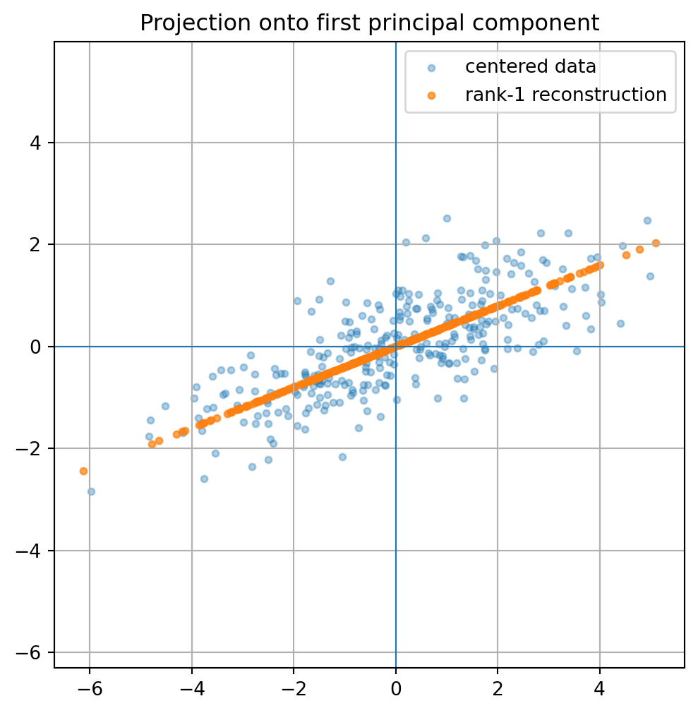
26.37 37. Quadratic forms
For a symmetric matrix \(A\), evaluate:
\[ q(x)=x^TAx. \]
A = np.array([[3, 1],
              [1, 2]], dtype=float)

x = np.array([1, 2], dtype=float)

x.T @ A @ x15.0For one-dimensional arrays, x.T is the same shape as x, but the expression works because NumPy treats it appropriately in dot products.
26.38 38. Plotting quadratic forms
def plot_quadratic_contours(A, title, xlim=(-3, 3), ylim=(-3, 3)):
    x = np.linspace(xlim[0], xlim[1], 250)
    y = np.linspace(ylim[0], ylim[1], 250)
    X, Y = np.meshgrid(x, y)

    Z = (
        A[0, 0] * X**2
        + (A[0, 1] + A[1, 0]) * X * Y
        + A[1, 1] * Y**2
    )

    plt.figure(figsize=(6, 6))
    cs = plt.contour(X, Y, Z, levels=18)
    plt.clabel(cs, inline=True, fontsize=8)
    plt.axhline(0, linewidth=0.8)
    plt.axvline(0, linewidth=0.8)
    plt.grid(True)
    plt.axis("equal")
    plt.title(title)
    plt.show()

A = np.array([[3, 1],
              [1, 2]], dtype=float)

plot_quadratic_contours(A, "$x^T A x$")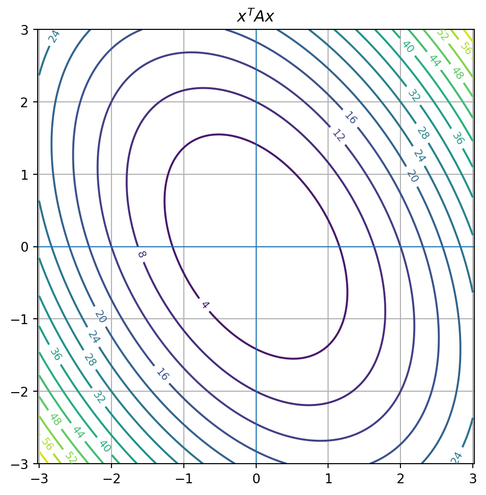
26.39 39. Classifying symmetric matrices by eigenvalues
def classify_symmetric(A, tol=1e-10):
    eigvals = np.linalg.eigvalsh(A)

    if np.all(eigvals > tol):
        kind = "positive definite"
    elif np.all(eigvals >= -tol):
        kind = "positive semidefinite"
    elif np.all(eigvals < -tol):
        kind = "negative definite"
    elif np.all(eigvals <= tol):
        kind = "negative semidefinite"
    else:
        kind = "indefinite"

    return eigvals, kind

A = np.array([[3, 1],
              [1, 2]], dtype=float)

classify_symmetric(A)
(array([1.38196601, 3.61803399]), 'positive definite')26.40 40. Gradient descent for a quadratic
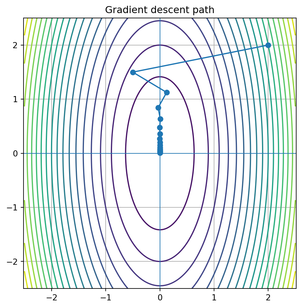
For
\[ f(x)=\frac12x^TAx-b^Tx, \]
the gradient is
\[ \nabla f(x)=Ax-b. \]
def gradient_descent_quadratic(A, b, x0, alpha, steps):
    x = x0.astype(float).copy()
    path = [x.copy()]

    for _ in range(steps):
        grad = A @ x - b
        x = x - alpha * grad
        path.append(x.copy())

    return np.array(path)

A = np.array([[5, 0],
              [0, 1]], dtype=float)

b = np.array([0, 0], dtype=float)

path = gradient_descent_quadratic(
    A=A,
    b=b,
    x0=np.array([2.0, 2.0]),
    alpha=0.25,
    steps=20
)

path[:5]
array([[ 2. , 2. ],
[-0.5 , 1.5 ],
[ 0.125 , 1.125 ],
[-0.03125 , 0.84375 ],
[ 0.0078125, 0.6328125]])Plot the path:
plot_quadratic_contours(A, "Gradient descent on a quadratic")

plt.figure(figsize=(6, 6))
x_grid = np.linspace(-2.5, 2.5, 250)
y_grid = np.linspace(-2.5, 2.5, 250)
Xg, Yg = np.meshgrid(x_grid, y_grid)
Zg = 0.5 * (A[0, 0] * Xg**2 + A[1, 1] * Yg**2)

cs = plt.contour(Xg, Yg, Zg, levels=20)
plt.plot(path[:, 0], path[:, 1], marker="o")
plt.axhline(0, linewidth=0.8)
plt.axvline(0, linewidth=0.8)
plt.grid(True)
plt.axis("equal")
plt.title("Gradient descent path")
plt.show()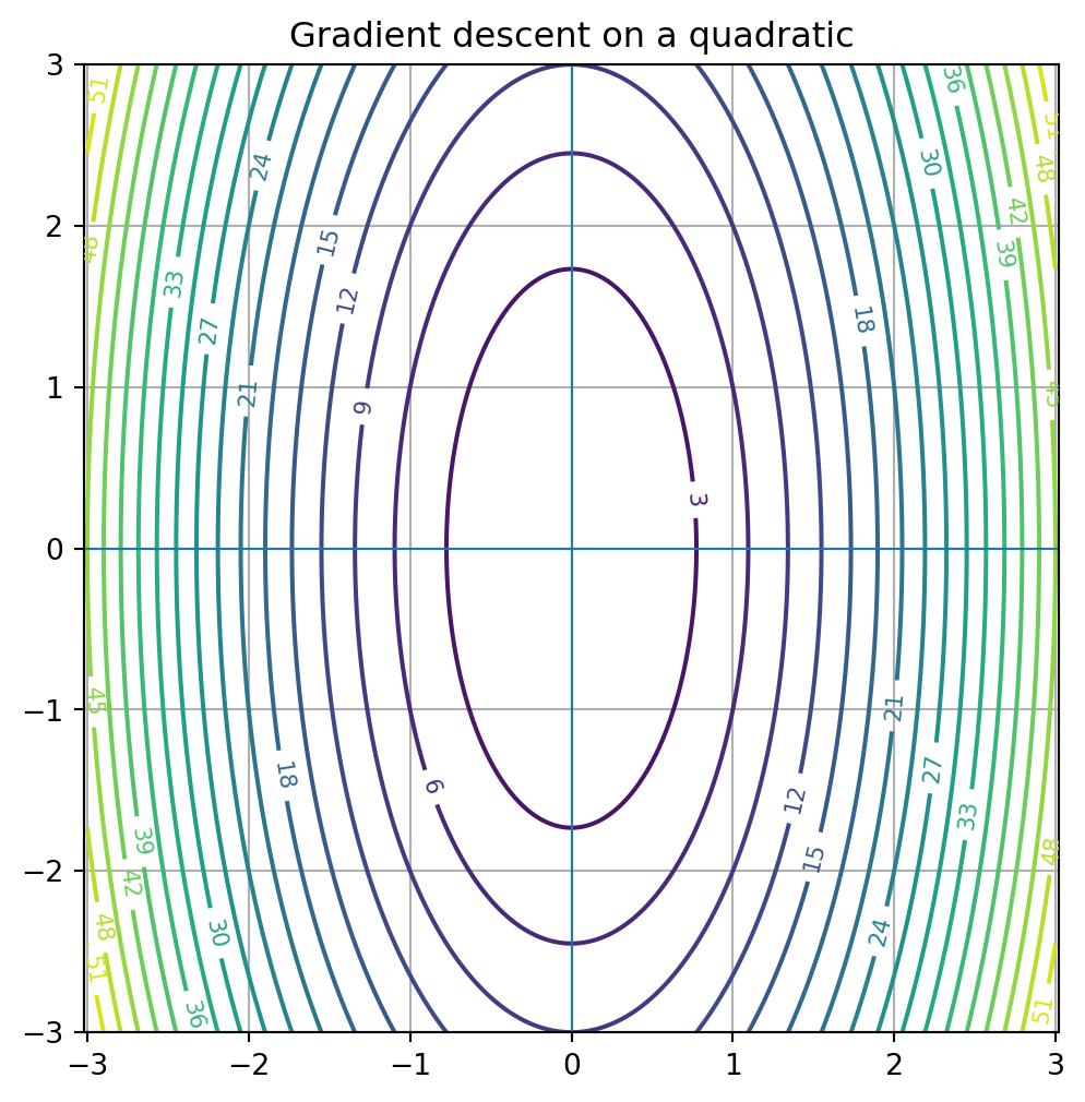
26.41 41. Plotting vectors in \(\\mathbb{R}^2\)
def plot_vector(v, label=None):
    plt.arrow(0, 0, v[0], v[1], head_width=0.08, length_includes_head=True)
    if label is not None:
        plt.text(v[0] + 0.05, v[1] + 0.05, label)

v = np.array([2, 1], dtype=float)
w = np.array([-1, 2], dtype=float)

plt.figure(figsize=(6, 6))
plot_vector(v, "$v$")
plot_vector(w, "$w$")
plt.axhline(0, linewidth=0.8)
plt.axvline(0, linewidth=0.8)
plt.grid(True)
plt.axis("equal")
plt.title("Vectors in $\\mathbb{R}^2$")
plt.show()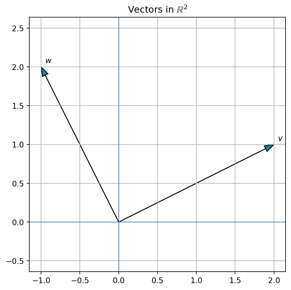
26.42 42. Plotting a linear transformation of a grid
def plot_transformed_grid(A, grid_lim=2, num_lines=9):
    values = np.linspace(-grid_lim, grid_lim, num_lines)

    plt.figure(figsize=(7, 7))

    for c in values:
        # vertical grid line
        y = np.linspace(-grid_lim, grid_lim, 200)
        x = np.full_like(y, c)
        points = np.vstack([x, y])
        transformed = A @ points
        plt.plot(transformed[0], transformed[1], linewidth=0.8)

        # horizontal grid line
        x = np.linspace(-grid_lim, grid_lim, 200)
        y = np.full_like(x, c)
        points = np.vstack([x, y])
        transformed = A @ points
        plt.plot(transformed[0], transformed[1], linewidth=0.8)

    plt.axhline(0, linewidth=0.8)
    plt.axvline(0, linewidth=0.8)
    plt.grid(True)
    plt.axis("equal")
    plt.title("Transformed grid")
    plt.show()

A = np.array([[1, 1],
              [0, 1]], dtype=float)

plot_transformed_grid(A)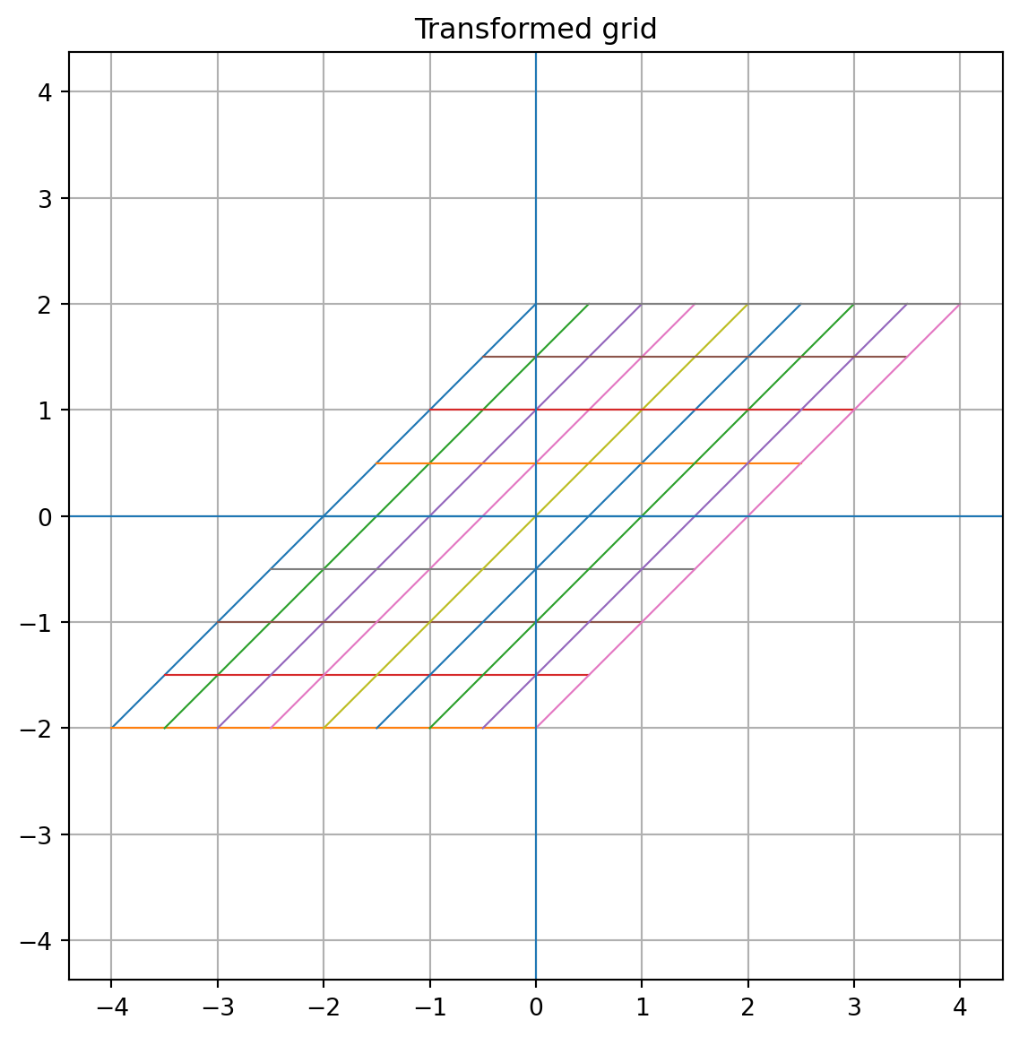
26.43 43. Plotting the unit circle and its image
def plot_circle_image(A):
    theta = np.linspace(0, 2*np.pi, 400)
    circle = np.vstack([np.cos(theta), np.sin(theta)])
    image = A @ circle

    plt.figure(figsize=(6, 6))
    plt.plot(circle[0], circle[1], label="unit circle")
    plt.plot(image[0], image[1], label="image under A")
    plt.axhline(0, linewidth=0.8)
    plt.axvline(0, linewidth=0.8)
    plt.grid(True)
    plt.axis("equal")
    plt.legend()
    plt.title("Unit circle and image")
    plt.show()

A = np.array([[2, 1],
              [0, 1]], dtype=float)

plot_circle_image(A)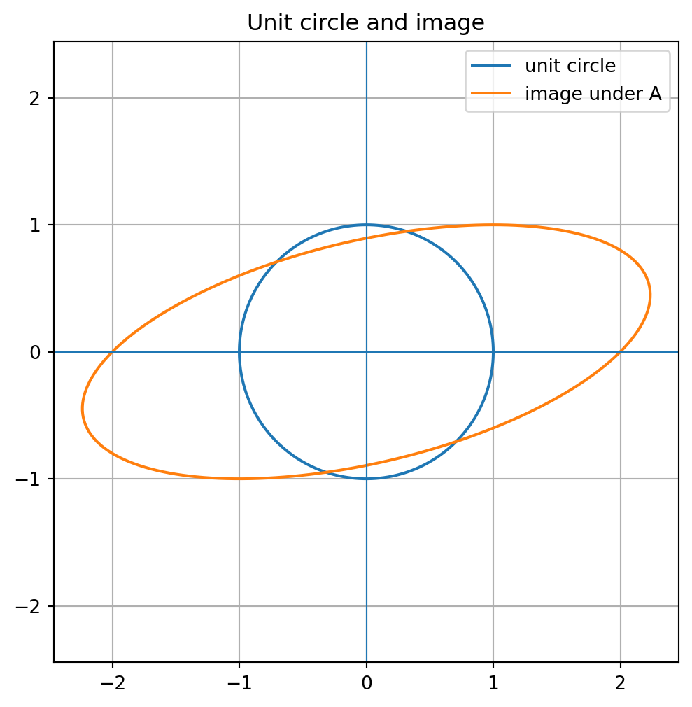
26.44 44. Random numbers and reproducibility
Use a random number generator with a seed.
rng = np.random.default_rng(0)

x = rng.normal(size=5)
x
array([ 0.12573022, -0.13210486, 0.64042265, 0.10490012, -0.53566937])Random matrix:
A = rng.normal(size=(3, 3))
A
array([[ 0.36159505, 1.30400005, 0.94708096],
[-0.70373524, -1.26542147, -0.62327446],
[ 0.04132598, -2.32503077, -0.21879166]])Random multivariate normal data:
X = rng.multivariate_normal(
    mean=[0, 0],
    cov=[[4, 1.5], [1.5, 1]],
    size=100
)

X[:5]
array([[ 2.64693109, 0.60865258],
[ 1.15543204, 0.26791721],
[-1.06303754, 0.25406354],
[-0.06650975, 0.88261269],
[ 1.23835713, 0.74707504]])Using a seed makes the example reproducible.
26.45 45. Working with data frames
For small tabular data, use pandas.
import pandas as pd

df = pd.DataFrame({
    "height": [65, 70, 68, 72],
    "weight": [130, 170, 155, 180],
    "age": [20, 22, 21, 23]
})

df| height | weight | age | |
|---|---|---|---|
| 0 | 65 | 130 | 20 |
| 1 | 70 | 170 | 22 |
| 2 | 68 | 155 | 21 |
| 3 | 72 | 180 | 23 |
Convert selected columns to a NumPy matrix:
X = df[["height", "weight", "age"]].to_numpy(dtype=float)
X
array([[ 65., 130., 20.],
[ 70., 170., 22.],
[ 68., 155., 21.],
[ 72., 180., 23.]])Column means:
X.mean(axis=0)array([ 68.75, 158.75, 21.5 ])Centered matrix:
Xc = X - X.mean(axis=0)
Xc
array([[ -3.75, -28.75, -1.5 ],
[ 1.25, 11.25, 0.5 ],
[ -0.75, -3.75, -0.5 ],
[ 3.25, 21.25, 1.5 ]])26.46 46. Common NumPy mistakes
26.46.1 Mistake 1: using * for matrix multiplication
Wrong for matrix multiplication:
A * BCorrect:
A @ B26.46.2 Mistake 2: forgetting dimensions
Check:
A.shape
B.shape
before multiplying.
26.46.3 Mistake 3: using inverse when solve is better
Prefer:
np.linalg.solve(A, b)over:
np.linalg.inv(A) @ b26.46.4 Mistake 4: expecting exact zeros
Numerical computations may produce tiny roundoff errors.
Use:
np.allclose(A @ x, b)instead of exact equality.
26.46.5 Mistake 5: confusing rows and columns in SVD
np.linalg.svd(A, full_matrices=False) returns:
U, s, VtThe right singular vectors are columns of:
V = Vt.T26.46.6 Mistake 6: using eig for symmetric matrices
For symmetric matrices, prefer:
np.linalg.eigh(A)over:
np.linalg.eig(A)26.47 47. Useful helper functions
26.47.1 Check symmetry
def is_symmetric(A, tol=1e-10):
    return np.linalg.norm(A - A.T) < tol
26.47.2 Check orthogonality
def is_orthogonal(Q, tol=1e-10):
    n = Q.shape[0]
    return np.linalg.norm(Q.T @ Q - np.eye(n)) < tol
26.47.3 Projection onto a line
def project_onto_line(b, a):
    return (np.dot(a, b) / np.dot(a, a)) * a
26.47.4 Unit vector
def unit_vector(x):
    return x / np.linalg.norm(x)
26.47.5 Rank-\(k\) approximation
def truncated_svd_approx(A, k):
    U, s, Vt = np.linalg.svd(A, full_matrices=False)
    return (U[:, :k] * s[:k]) @ Vt[:k, :]
26.47.6 Center a data matrix
def center_columns(X):
    return X - X.mean(axis=0)
26.47.7 Standardize a data matrix
def standardize_columns(X):
    Xc = X - X.mean(axis=0)
    return Xc / Xc.std(axis=0, ddof=1)
26.48 48. Mini-project patterns
26.48.1 Pattern 1: solve and interpret a system
A = ...
b = ...

x = np.linalg.solve(A, b)
residual = b - A @ x
Questions:
- Is the solution exact?
- What do the entries of \(x\) mean?
- Is the matrix invertible?
- Is the system well-conditioned?
26.48.2 Pattern 2: fit a least-squares model
A = ...
b = ...

x_hat = np.linalg.lstsq(A, b, rcond=None)[0]
b_hat = A @ x_hat
residual = b - b_hat
Questions:
- What model space is being used?
- What is the residual?
- Is the residual orthogonal to the column space?
- How good is the fit?
26.48.3 Pattern 3: analyze a transformation
A = ...

det_A = np.linalg.det(A)
rank_A = np.linalg.matrix_rank(A)
eigvals = np.linalg.eigvals(A)
singular_values = np.linalg.svd(A, compute_uv=False)
Questions:
- Is the transformation invertible?
- Does it preserve or collapse area?
- What are its eigen-directions?
- What are its singular values?
26.48.4 Pattern 4: analyze data with PCA
X = ...
Xc = X - X.mean(axis=0)

U, s, Vt = np.linalg.svd(Xc, full_matrices=False)

V = Vt.T
explained_variance = s**2 / (len(Xc) - 1)
Questions:
- What are the principal directions?
- How much variance does each direction explain?
- Is the data approximately low-dimensional?
- What is the reconstruction error after projection?
26.49 49. Recommended computational habits
- Always check matrix shapes.
- Use
@for matrix multiplication. - Prefer
solveover explicit inverse. - Prefer
lstsq, QR, or SVD for least-squares problems. - Use
eighfor symmetric matrices. - Use SVD for rank, conditioning, low-rank approximation, and PCA.
- Use
np.allclosefor numerical equality. - Plot whenever geometry matters.
- Use random seeds for reproducibility.
- Interpret numerical output mathematically.
26.50 50. Final reference table
| Task | Python command |
|---|---|
| Matrix multiplication | A @ B |
| Matrix-vector product | A @ x |
| Transpose | A.T |
| Identity matrix | np.eye(n) |
| Zero matrix | np.zeros((m, n)) |
| Diagonal matrix | np.diag(values) |
| Dot product | np.dot(x, y) or x @ y |
| Norm | np.linalg.norm(x) |
| Solve \(Ax=b\) | np.linalg.solve(A, b) |
| Least squares | np.linalg.lstsq(A, b, rcond=None) |
| Inverse | np.linalg.inv(A) |
| Determinant | np.linalg.det(A) |
| Rank | np.linalg.matrix_rank(A) |
| QR factorization | np.linalg.qr(A, mode="reduced") |
| Eigenvalues | np.linalg.eigvals(A) |
| Eigenpairs | np.linalg.eig(A) |
| Symmetric eigenpairs | np.linalg.eigh(A) |
| SVD | np.linalg.svd(A, full_matrices=False) |
| Singular values only | np.linalg.svd(A, compute_uv=False) |
| Pseudoinverse | np.linalg.pinv(A) |
| Condition number | np.linalg.cond(A) |
| RREF | sp.Matrix(A).rref() |
| Exact null space | sp.Matrix(A).nullspace() |
| Exact column space | sp.Matrix(A).columnspace() |
26.51 Closing note
Python is a laboratory for linear algebra.
Use it to compute, visualize, test, and explore. But always connect the output back to the mathematics:
- What is the matrix doing?
- What subspace is being described?
- What geometry is being preserved or changed?
- What approximation is being made?
- What structure is hidden in the data?
The purpose of computation is understanding.