Opening question
Some matrices distort space. They stretch, shear, collapse, and twist vectors in complicated ways.
Other matrices are more structured.
An orthogonal matrix preserves lengths and angles. It moves space rigidly, like a rotation or reflection.
A symmetric matrix has a different kind of structure. It satisfies
\[
A^T=A.
\]
Symmetric matrices are central because their eigenvectors can be chosen orthonormally and their eigenvalues are real. This leads to the spectral theorem , one of the most important results in linear algebra.
The central question of this chapter is:
Which matrices have the best geometric and spectral structure?
Orthogonal matrices preserve geometry. Symmetric matrices reveal geometry.
Together, they prepare the way for quadratic forms, the spectral theorem, PCA, and the singular value decomposition.
Learning goals
After studying this chapter, you should be able to:
Define orthogonal matrices.
Recognize rotations and reflections as orthogonal matrices.
Prove that orthogonal matrices preserve lengths and dot products.
Understand why \(Q^{-1}=Q^T\) for orthogonal matrices.
Define symmetric matrices.
Compute eigenvalues and eigenvectors of symmetric matrices.
Understand why eigenvectors of symmetric matrices are orthogonal.
State and use the spectral theorem for real symmetric matrices.
Diagonalize a symmetric matrix using an orthogonal matrix.
Use Python to visualize and compute orthogonal and symmetric matrix structure.
19.1 Orthogonal matrices
A square matrix \(Q\) is called orthogonal if its columns form an orthonormal basis of \(\mathbb{R}^n\) .
This means:
\[
q_i\cdot q_j=0
\]
for \(i\ne j\) , and
\[
q_i\cdot q_i=1
\]
for every \(i\) .
In matrix form, this condition is
\[
Q^TQ=I.
\]
A square matrix \(Q\) is orthogonal if
\[
Q^TQ=I.
\]
Since \(Q\) is square, this also implies
\[
QQ^T=I.
\]
Therefore
\[
Q^{-1}=Q^T.
\]
This is the key algebraic advantage of orthogonal matrices.
If \(Q\) is orthogonal, then
\[
Q^{-1}=Q^T.
\]
19.2 Examples of orthogonal matrices
The identity matrix
The identity matrix
\[
I=
\begin{bmatrix}
1&0\\
0&1
\end{bmatrix}
\]
is orthogonal because
\[
I^TI=I.
\]
Rotation matrices
For an angle \(\theta\) ,
\[
Q=
\begin{bmatrix}
\cos\theta&-\sin\theta\\
\sin\theta&\cos\theta
\end{bmatrix}
\]
is orthogonal.
Its columns are
\[
q_1=
\begin{bmatrix}
\cos\theta\\
\sin\theta
\end{bmatrix},
\qquad
q_2=
\begin{bmatrix}
-\sin\theta\\
\cos\theta
\end{bmatrix}.
\]
They have length \(1\) and are orthogonal:
\[
q_1\cdot q_2
=
-\cos\theta\sin\theta+\sin\theta\cos\theta
=
0.
\]
Reflection matrices
The matrix
\[
Q=
\begin{bmatrix}
1&0\\
0&-1
\end{bmatrix}
\]
reflects across the \(x\) -axis.
It is orthogonal because
\[
Q^TQ=
\begin{bmatrix}
1&0\\
0&-1
\end{bmatrix}
\begin{bmatrix}
1&0\\
0&-1
\end{bmatrix}
=
I.
\]
19.3 Orthogonal matrices preserve length
Let \(Q\) be orthogonal. Then for every vector \(x\) ,
\[
\|Qx\|^2=(Qx)^T(Qx).
\]
Using transpose rules,
\[
(Qx)^T(Qx)=x^TQ^TQx.
\]
Since \(Q^TQ=I\) ,
\[
x^TQ^TQx=x^TIx=x^Tx=\|x\|^2.
\]
Thus
\[
\|Qx\|=\|x\|.
\]
If \(Q\) is orthogonal, then
\[
\|Qx\|=\|x\|
\]
for every vector \(x\) .
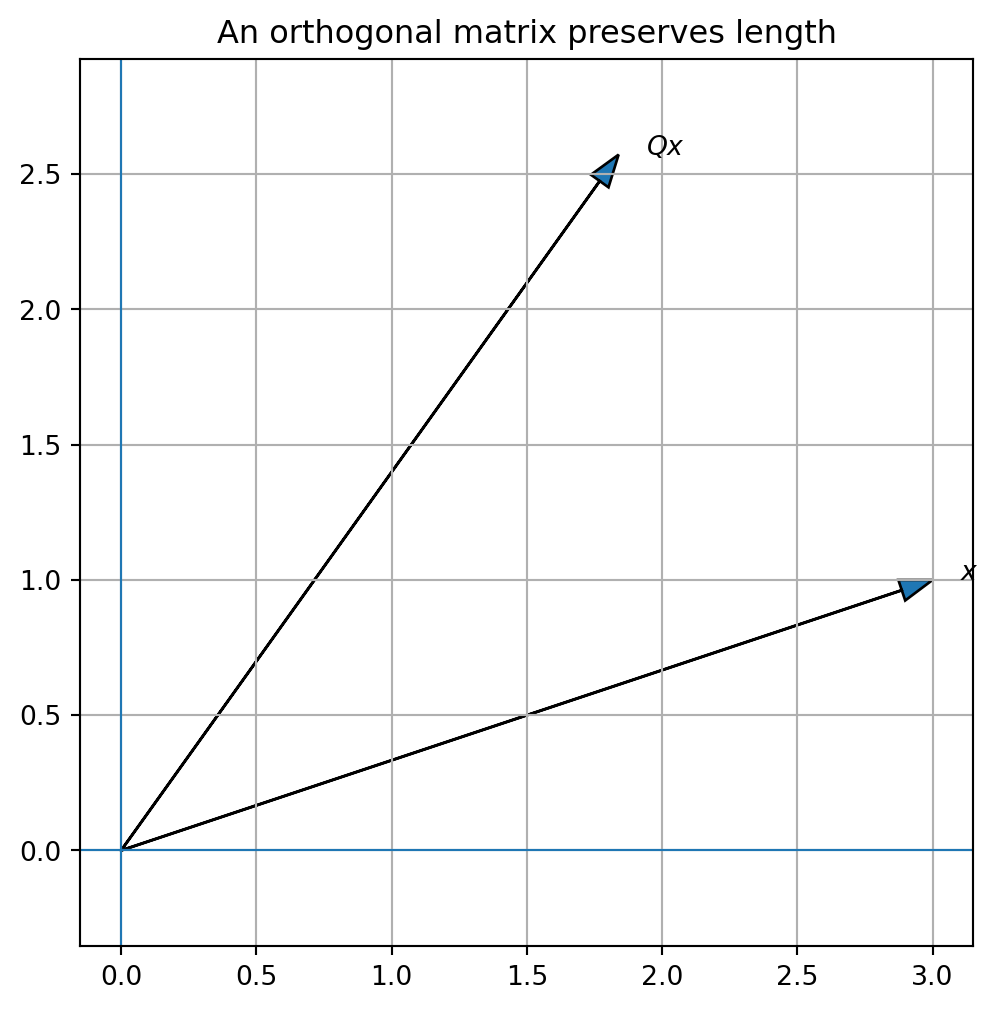
Orthogonal matrices do not stretch or shrink vectors. They preserve distances from the origin.
19.4 Orthogonal matrices preserve dot products
Let \(Q\) be orthogonal. Then
\[
(Qx)\cdot(Qy)=(Qx)^T(Qy).
\]
So
\[
(Qx)^T(Qy)=x^TQ^TQy=x^Ty=x\cdot y.
\]
Thus
\[
(Qx)\cdot(Qy)=x\cdot y.
\]
If \(Q\) is orthogonal, then
\[
(Qx)\cdot(Qy)=x\cdot y
\]
for all vectors \(x\) and \(y\) .
Since lengths and dot products are preserved, angles are preserved as well.
Orthogonal transformations are rigid motions fixing the origin: rotations, reflections, and combinations of them.
19.5 Python plot: rotation preserves length
import numpy as npimport matplotlib.pyplot as plt= np.pi / 5 = np.array([- np.sin(theta)],= np.array([3 , 1 ], dtype= float )= Q @ x= (6 , 6 ))0 , 0 , x[0 ], x[1 ], head_width= 0.08 , length_includes_head= True )0 , 0 , Qx[0 ], Qx[1 ], head_width= 0.08 , length_includes_head= True )0 ] + 0.1 , x[1 ], "$x$" )0 ] + 0.1 , Qx[1 ], "$Qx$" )0 , linewidth= 0.8 )0 , linewidth= 0.8 )True )"equal" )"An orthogonal matrix preserves length" )@ Q
(3.1622776601683795,
 3.1622776601683795,
 array([[ 1.00000000e+00, -1.26599665e-17],
        [-1.26599665e-17,  1.00000000e+00]]))
19.6 Determinant of an orthogonal matrix
If \(Q\) is orthogonal, then
\[
Q^TQ=I.
\]
Take determinants:
\[
\det(Q^TQ)=\det(I).
\]
Using determinant properties,
\[
\det(Q^T)\det(Q)=1.
\]
Since
\[
\det(Q^T)=\det(Q),
\]
we get
\[
(\det Q)^2=1.
\]
Therefore
\[
\det(Q)=1
\]
or
\[
\det(Q)=-1.
\]
If \(Q\) is orthogonal, then
\[
\det(Q)=\pm 1.
\]
When \(\det(Q)=1\) , the transformation preserves orientation. Rotations have determinant \(1\) .
When \(\det(Q)=-1\) , the transformation reverses orientation. Reflections have determinant \(-1\) .
19.7 Orthogonal matrices and coordinates
If \(Q\) is orthogonal, then converting coordinates using \(Q\) is stable.
Because
\[
Q^{-1}=Q^T,
\]
we can recover \(x\) from \(Qx\) by applying \(Q^T\) :
\[
x=Q^T(Qx).
\]
This is computationally important. Multiplication by an orthogonal matrix does not magnify errors in length.
For this reason, numerical algorithms often prefer orthogonal transformations.
QR factorization, Householder reflections, and many eigenvalue algorithms are built from orthogonal matrices.
19.8 Symmetric matrices
A square matrix \(A\) is symmetric if
\[
A^T=A.
\]
This means that entries mirror across the main diagonal:
\[
a_{ij}=a_{ji}.
\]
A square matrix \(A\) is symmetric if
\[
A^T=A.
\]
Examples:
\[
\begin{bmatrix}
2&1\\
1&3
\end{bmatrix}
\]
is symmetric.
\[
\begin{bmatrix}
1&4&0\\
4&2&-1\\
0&-1&5
\end{bmatrix}
\]
is symmetric.
But
\[
\begin{bmatrix}
1&2\\
3&4
\end{bmatrix}
\]
is not symmetric.
19.9 Why symmetric matrices matter
Symmetric matrices appear naturally in many places:
covariance matrices,
Gram matrices \(A^TA\) ,
Hessian matrices of second derivatives,
graph adjacency matrices for undirected graphs,
graph Laplacian matrices,
quadratic forms,
least-squares normal equations,
PCA and spectral decomposition.
The reason symmetric matrices are so important is spectral structure.
For real symmetric matrices:
all eigenvalues are real,
eigenvectors corresponding to distinct eigenvalues are orthogonal,
there is an orthonormal basis of eigenvectors,
the matrix can be diagonalized by an orthogonal matrix.
These facts make symmetric matrices among the best-behaved matrices in linear algebra.
19.10 Example: eigenvectors of a symmetric matrix
Let
\[
A=
\begin{bmatrix}
2&1\\
1&2
\end{bmatrix}.
\]
This matrix is symmetric.
We already found eigenvectors
\[
v_1=
\begin{bmatrix}
1\\
1
\end{bmatrix}
\]
with eigenvalue \(3\) , and
\[
v_2=
\begin{bmatrix}
1\\
-1
\end{bmatrix}
\]
with eigenvalue \(1\) .
Notice that
\[
v_1\cdot v_2
=
\begin{bmatrix}
1\\
1
\end{bmatrix}
\cdot
\begin{bmatrix}
1\\
-1
\end{bmatrix}
=
1-1=0.
\]
The eigenvectors are orthogonal.
After normalizing,
\[
q_1=\frac{1}{\sqrt{2}}
\begin{bmatrix}
1\\
1
\end{bmatrix},
\qquad
q_2=\frac{1}{\sqrt{2}}
\begin{bmatrix}
1\\
-1
\end{bmatrix}.
\]
Then \(q_1,q_2\) form an orthonormal eigenbasis.
19.11 Eigenvectors for distinct eigenvalues are orthogonal
Let \(A\) be symmetric.
Suppose
\[
Av=\lambda v
\]
and
\[
Aw=\mu w,
\]
where
\[
\lambda\ne \mu.
\]
We prove that
\[
v\cdot w=0.
\]
Start with
\[
(Av)\cdot w.
\]
Since \(Av=\lambda v\) ,
\[
(Av)\cdot w=(\lambda v)\cdot w=\lambda(v\cdot w).
\]
On the other hand,
\[
(Av)\cdot w=(Av)^Tw=v^TA^Tw.
\]
Because \(A\) is symmetric,
\[
A^T=A.
\]
So
\[
v^TA^Tw=v^TAw=v\cdot(Aw).
\]
Since \(Aw=\mu w\) ,
\[
v\cdot(Aw)=v\cdot(\mu w)=\mu(v\cdot w).
\]
Therefore
\[
\lambda(v\cdot w)=\mu(v\cdot w).
\]
So
\[
(\lambda-\mu)(v\cdot w)=0.
\]
Since \(\lambda\ne\mu\) ,
\[
v\cdot w=0.
\]
For a symmetric matrix, eigenvectors corresponding to distinct eigenvalues are orthogonal.
19.12 Python: symmetric eigenvectors
= np.array([[2 , 1 ],1 , 2 ]], dtype= float )= np.linalg.eigh(A)@ eigvecs
(array([1., 3.]),
 array([[-0.70710678,  0.70710678],
        [ 0.70710678,  0.70710678]]),
 array([[1.00000000e+00, 2.23711432e-17],
        [2.23711432e-17, 1.00000000e+00]]))
The function np.linalg.eigh is designed for symmetric or Hermitian matrices.
It returns orthonormal eigenvectors.
The output eigvecs.T @ eigvecs should be close to the identity matrix.
19.13 Orthogonal diagonalization
If \(A\) is symmetric, then \(A\) can be diagonalized using an orthogonal matrix.
That means there exists an orthogonal matrix \(Q\) and a diagonal matrix \(D\) such that
\[
A=QDQ^T.
\]
Equivalently,
\[
Q^TAQ=D.
\]
This is a special and stronger form of diagonalization.
For a general diagonalizable matrix, we write
\[
A=PDP^{-1}.
\]
For a symmetric matrix, the eigenvector matrix can be chosen orthogonal, so
\[
P^{-1}=P^T.
\]
Thus
\[
A=QDQ^T.
\]
A matrix \(A\) is orthogonally diagonalizable if there exists an orthogonal matrix \(Q\) and a diagonal matrix \(D\) such that
\[
A=QDQ^T.
\]
19.14 The spectral theorem
The central theorem for symmetric matrices is the spectral theorem.
If \(A\) is a real symmetric matrix, then there exists an orthogonal matrix \(Q\) and a real diagonal matrix \(D\) such that
\[
A=QDQ^T.
\]
The columns of \(Q\) are orthonormal eigenvectors of \(A\) , and the diagonal entries of \(D\) are the corresponding real eigenvalues.
This theorem says:
Every real symmetric matrix has an orthonormal eigenbasis.
That is one of the most powerful structural results in linear algebra.
19.15 Example: orthogonal diagonalization
Let
\[
A=
\begin{bmatrix}
2&1\\
1&2
\end{bmatrix}.
\]
Use orthonormal eigenvectors
\[
q_1=
\frac{1}{\sqrt{2}}
\begin{bmatrix}
1\\
1
\end{bmatrix},
\qquad
q_2=
\frac{1}{\sqrt{2}}
\begin{bmatrix}
1\\
-1
\end{bmatrix}.
\]
Let
\[
Q=
\frac{1}{\sqrt{2}}
\begin{bmatrix}
1&1\\
1&-1
\end{bmatrix},
\]
and
\[
D=
\begin{bmatrix}
3&0\\
0&1
\end{bmatrix}.
\]
Then
\[
A=QDQ^T.
\]
Equivalently,
\[
Q^TAQ=D.
\]
19.16 Python: orthogonal diagonalization
= np.array([[2 , 1 ],1 , 2 ]], dtype= float )= np.linalg.eigh(A)= np.diag(eigvals)@ A @ Q, D, Q @ D @ Q.T
(array([[ 1.00000000e+00,  2.23711432e-17],
        [-4.39088730e-17,  3.00000000e+00]]),
 array([[1., 0.],
        [0., 3.]]),
 array([[2., 1.],
        [1., 2.]]))
The reconstruction \(QDQ^T\) should equal \(A\) up to numerical roundoff.
19.17 Spectral decomposition as a sum of projections
If
\[
A=QDQ^T,
\]
where
\[
Q=\begin{bmatrix}q_1&q_2&\cdots&q_n\end{bmatrix}
\]
and
\[
D=\operatorname{diag}(\lambda_1,\ldots,\lambda_n),
\]
then
\[
A=\lambda_1q_1q_1^T+\lambda_2q_2q_2^T+\cdots+\lambda_nq_nq_n^T.
\]
Each matrix
\[
q_iq_i^T
\]
is the projection matrix onto the line spanned by \(q_i\) .
So a symmetric matrix is a weighted sum of orthogonal projection matrices.
For a real symmetric matrix,
\[
A=\sum_{i=1}^n \lambda_i q_iq_i^T.
\]
This formula is extremely important for PCA, covariance matrices, quadratic forms, and the SVD.
19.18 Python: spectral decomposition
= np.array([[2 , 1 ],1 , 2 ]], dtype= float )= np.linalg.eigh(A)= np.zeros_like(A)for i in range (len (eigvals)):= Q[:, i:i+ 1 ]+= eigvals[i] * (q @ q.T)
(array([[2., 1.],
        [1., 2.]]),
 array([[2., 1.],
        [1., 2.]]))
The sum reconstructs the matrix.
19.20 Positive definite matrices preview
A symmetric matrix \(A\) is positive definite if
\[
x^TAx>0
\]
for every nonzero vector \(x\) .
For symmetric matrices, positive definiteness is determined by eigenvalues.
A symmetric matrix is positive definite if and only if all eigenvalues are positive.
It is positive semidefinite if and only if all eigenvalues are nonnegative.
These ideas will appear in the chapter on quadratic forms.
19.21 Gram matrices are symmetric
For any matrix \(A\) , the matrix
\[
A^TA
\]
is symmetric because
\[
(A^TA)^T=A^T(A^T)^T=A^TA.
\]
Also, for any vector \(x\) ,
\[
x^T(A^TA)x=(Ax)^T(Ax)=\|Ax\|^2\ge 0.
\]
Thus \(A^TA\) is positive semidefinite.
If the columns of \(A\) are linearly independent, then
\[
\|Ax\|^2>0
\]
for every nonzero \(x\) , so \(A^TA\) is positive definite.
This explains why \(A^TA\) plays such an important role in least squares.
19.22 Covariance matrices and PCA preview
In data analysis, covariance matrices are symmetric.
A covariance matrix measures how variables vary together.
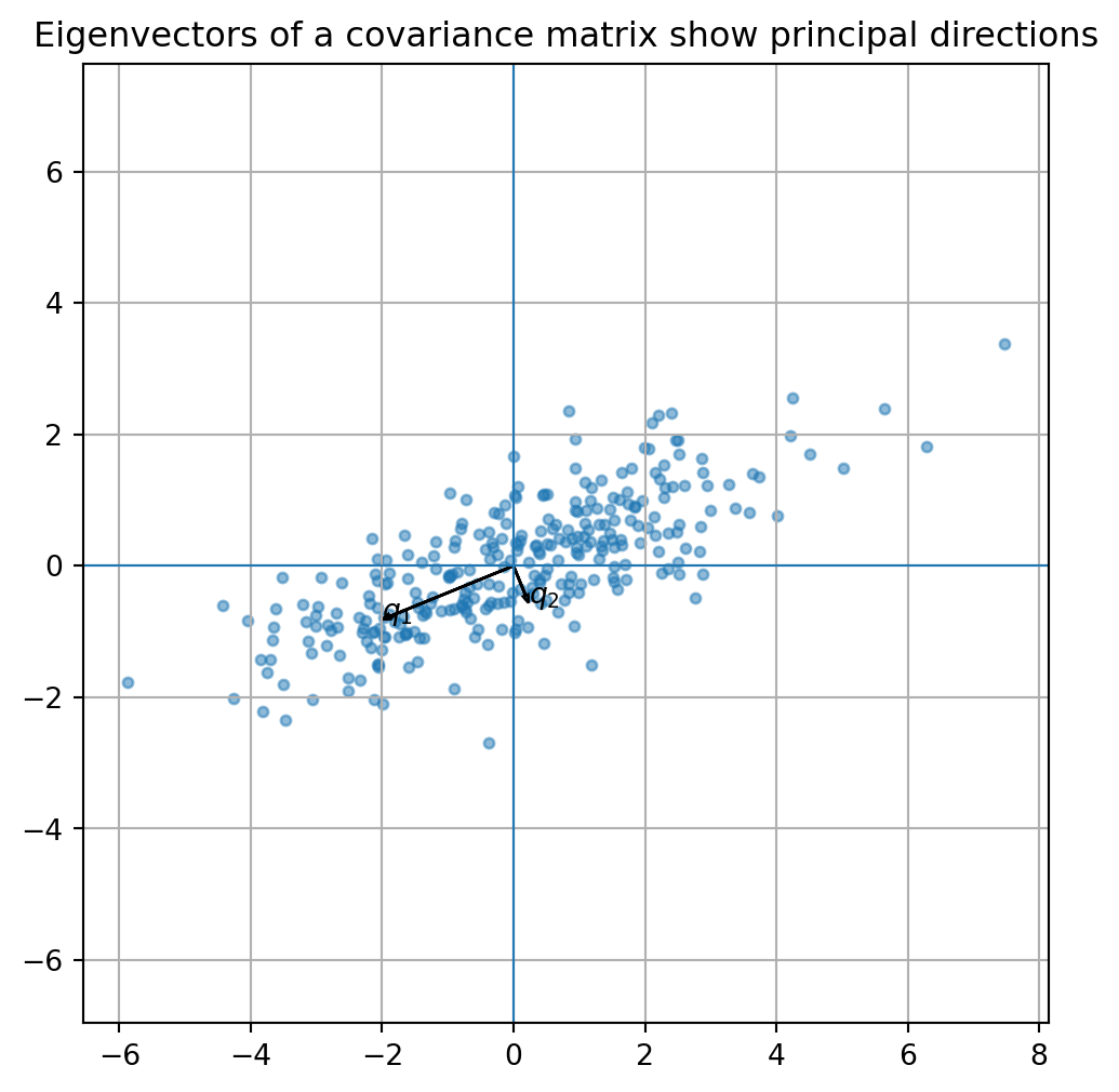
Its eigenvectors give principal directions of variation.
Its eigenvalues measure how much variation occurs in those directions.
This is the foundation of principal component analysis.
In PCA:
eigenvectors of a covariance matrix become principal components,
eigenvalues measure explained variance,
orthogonality ensures that principal directions are uncorrelated.
19.23 Python: covariance eigenvectors
= np.random.default_rng(0 )= rng.multivariate_normal(= [0 , 0 ],= [[4 , 1.5 ], [1.5 , 1 ]],= 300 # Center the data = X - X.mean(axis= 0 )# Sample covariance matrix = X_centered.T @ X_centered / (len (X_centered) - 1 )= np.linalg.eigh(C)# Sort descending = np.argsort(eigvals)[::- 1 ]= eigvals[idx]= Q[:, idx]= (6 , 6 ))0 ], X_centered[:, 1 ], s= 12 , alpha= 0.5 )for i in range (2 ):= Q[:, i]= np.sqrt(eigvals[i])0 , 0 , length* direction[0 ], length* direction[1 ],= 0.08 , length_includes_head= True )* direction[0 ], length* direction[1 ], f"$q_ { i+ 1 } $" )0 , linewidth= 0.8 )0 , linewidth= 0.8 )True )"equal" )"Eigenvectors of a covariance matrix show principal directions" )@ Q
(array([[4.05002023, 1.50312826],
        [1.50312826, 0.98378203]]),
 array([4.66395696, 0.3698453 ]),
 array([[ 1.00000000e+00, -1.72673896e-17],
        [-1.72673896e-17,  1.00000000e+00]]))
19.24 Symmetric matrices and optimization preview
If
\[
f(x)=\frac12x^TAx-b^Tx,
\]
where \(A\) is symmetric, then
\[
\nabla f(x)=Ax-b.
\]
If \(A\) is positive definite, then this function has a unique minimum.
The eigenvalues of \(A\) describe the shape of the energy landscape:
large eigenvalues mean steep curvature,
small eigenvalues mean shallow curvature,
negative eigenvalues indicate directions of downward curvature.
This connects symmetric matrices to optimization and machine learning.
19.25 Comparing orthogonal and symmetric matrices
Orthogonal matrices and symmetric matrices are different kinds of structure.
Orthogonal
\(Q^TQ=I\) preserves lengths and angles
Symmetric
\(A^T=A\) has real eigenvalues and orthogonal eigenspaces
Some matrices are both orthogonal and symmetric.
For example,
\[
F=
\begin{bmatrix}
1&0\\
0&-1
\end{bmatrix}
\]
is both symmetric and orthogonal.
It is a reflection.
If a matrix is both symmetric and orthogonal, then its eigenvalues are only
\[
1
\]
or
\[
-1.
\]
Why?
Orthogonal matrices have eigenvalues with absolute value \(1\) .
Symmetric matrices have real eigenvalues.
So the eigenvalues must be real numbers with absolute value \(1\) .
19.26 Python: comparing structures
def is_orthogonal(A, tol= 1e-10 ):= A.shape[0 ]return np.linalg.norm(A.T @ A - np.eye(n)) < toldef is_symmetric(A, tol= 1e-10 ):return np.linalg.norm(A.T - A) < tol= np.array([[0 , - 1 ],1 , 0 ]], dtype= float )= np.array([[1 , 0 ],0 , - 1 ]], dtype= float )= np.array([[2 , 1 ],1 , 2 ]], dtype= float )for name, M in [("rotation" , R), ("reflection" , F), ("symmetric" , S)]:print (name)print ("orthogonal:" , is_orthogonal(M))print ("symmetric:" , is_symmetric(M))print ("eigenvalues:" , np.linalg.eigvals(M))print ()
rotation
orthogonal: True
symmetric: False
eigenvalues: [0.+1.j 0.-1.j]

reflection
orthogonal: True
symmetric: True
eigenvalues: [ 1. -1.]

symmetric
orthogonal: False
symmetric: True
eigenvalues: [3. 1.]
19.27 Algorithmic summary
For a square matrix \(Q\) :
Compute \(Q^TQ\) .
If
\[
Q^TQ=I,
\]
then \(Q\) is orthogonal.
For a square matrix \(A\) :
Compute \(A^T\) .
If
\[
A^T=A,
\]
then \(A\) is symmetric.
For a symmetric matrix \(A\) :
Find eigenvalues and orthonormal eigenvectors.
Place orthonormal eigenvectors as columns of \(Q\) .
Place corresponding eigenvalues on the diagonal of \(D\) .
Then
\[
A=QDQ^T.
\]
If \(A\) is symmetric with orthonormal eigenvectors \(q_i\) and eigenvalues \(\lambda_i\) , then
\[
A=\sum_i \lambda_i q_iq_i^T.
\]
19.28 Common mistakes
Mistake 1: confusing orthogonal vectors and orthogonal matrices
Vectors are orthogonal when their dot product is zero.
A square matrix is orthogonal when its columns form an orthonormal basis, equivalently
\[
Q^TQ=I.
\]
Mistake 2: thinking orthogonal matrices have orthogonal rows only
For a square matrix, orthonormal columns imply orthonormal rows.
Both are true.
Mistake 3: forgetting that \(Q^{-1}=Q^T\)
This is the main computational advantage of orthogonal matrices.
Mistake 4: assuming every diagonalizable matrix is orthogonally diagonalizable
Only special matrices, especially real symmetric matrices, have orthonormal eigenvector bases.
Mistake 5: using np.linalg.eig when the matrix is symmetric
For symmetric matrices, use np.linalg.eigh, which is designed for symmetric eigenvalue problems and returns orthonormal eigenvectors.
Mistake 6: ignoring eigenvector order
In
\[
A=QDQ^T,
\]
the order of eigenvalues in \(D\) must match the order of eigenvectors in \(Q\) .
19.29 Chapter summary
An orthogonal matrix satisfies
\[
Q^TQ=I.
\]
For an orthogonal matrix,
\[
Q^{-1}=Q^T.
\]
Orthogonal matrices preserve lengths, dot products, distances, and angles.
Their determinants are
\[
\pm 1.
\]
A symmetric matrix satisfies
\[
A^T=A.
\]
Symmetric matrices have real eigenvalues and orthogonal eigenspaces.
The spectral theorem says that every real symmetric matrix can be written as
\[
A=QDQ^T,
\]
where \(Q\) is orthogonal and \(D\) is diagonal.
Equivalently,
\[
Q^TAQ=D.
\]
The spectral decomposition is
\[
A=\sum_i \lambda_i q_iq_i^T.
\]
Symmetric matrices appear in covariance matrices, least squares, quadratic forms, graph theory, optimization, PCA, and the SVD.
Exercises
A. Orthogonal matrices
Determine whether each matrix is orthogonal.
\[
\begin{bmatrix}
1&0\\
0&1
\end{bmatrix}
\]
\[
\begin{bmatrix}
0&-1\\
1&0
\end{bmatrix}
\]
\[
\begin{bmatrix}
1&0\\
0&-1
\end{bmatrix}
\]
\[
\frac{1}{\sqrt{2}}
\begin{bmatrix}
1&1\\
1&-1
\end{bmatrix}
\]
\[
\begin{bmatrix}
2&0\\
0&1/2
\end{bmatrix}
\]
B. Length and dot product preservation
For each orthogonal matrix in Exercise A, choose two vectors \(x\) and \(y\) and verify that
\[
\|Qx\|=\|x\|,
\]
and
\[
(Qx)\cdot(Qy)=x\cdot y.
\]
C. Symmetric matrices
Determine whether each matrix is symmetric.
\[
\begin{bmatrix}
2&1\\
1&3
\end{bmatrix}
\]
\[
\begin{bmatrix}
1&2\\
3&4
\end{bmatrix}
\]
\[
\begin{bmatrix}
1&4&0\\
4&2&-1\\
0&-1&5
\end{bmatrix}
\]
\[
\begin{bmatrix}
0&-1\\
1&0
\end{bmatrix}
\]
D. Orthogonal diagonalization
For each symmetric matrix:
Find eigenvalues.
Find an orthonormal eigenbasis.
Form \(Q\) and \(D\) .
Verify that \(A=QDQ^T\) .
\[
A=
\begin{bmatrix}
2&1\\
1&2
\end{bmatrix}
\]
\[
A=
\begin{bmatrix}
3&0\\
0&1
\end{bmatrix}
\]
\[
A=
\begin{bmatrix}
4&2\\
2&4
\end{bmatrix}
\]
E. Spectral decomposition
For
\[
A=
\begin{bmatrix}
2&1\\
1&2
\end{bmatrix},
\]
write \(A\) as
\[
A=\lambda_1q_1q_1^T+\lambda_2q_2q_2^T.
\]
F. Gram matrices
Let
\[
A=
\begin{bmatrix}
1&2\\
3&4\\
5&6
\end{bmatrix}.
\]
Compute \(A^TA\) .
Verify that \(A^TA\) is symmetric.
Compute \(x^T(A^TA)x\) for a nonzero vector \(x\) .
Explain why \(A^TA\) is positive semidefinite.
G. Python exercises
Write a function to test whether a matrix is orthogonal.
Write a function to test whether a matrix is symmetric.
Use np.linalg.eigh to diagonalize a symmetric matrix.
Verify \(A=QDQ^T\) numerically.
Build the spectral decomposition as a sum of \(\lambda_iq_iq_i^T\) .
Generate a random data set, compute its covariance matrix, and plot the eigenvectors.
Compare np.linalg.eig and np.linalg.eigh on a symmetric matrix.
H. Reflection
Write a short paragraph answering each question.
Why do orthogonal matrices preserve geometry?
Why is \(Q^{-1}=Q^T\) computationally useful?
Why are symmetric matrices better behaved than general matrices?
Why does the spectral theorem matter?
How do symmetric matrices appear in data science and AI?
AI-age connection
Orthogonal and symmetric matrices are central to reliable computation. Orthogonal matrices preserve geometry and numerical stability. Symmetric matrices reveal hidden directions through real eigenvalues and orthonormal eigenvectors. Covariance matrices, Gram matrices, graph Laplacians, Hessians, and attention-related similarity matrices all use symmetric structure. PCA, spectral clustering, optimization, and the SVD all depend on the ideas in this chapter.