Opening question
Suppose a vector \(b\) does not lie on a line or inside a subspace.
We may still want the closest vector in that line or subspace.
This is the idea of projection.
Projection answers questions such as:
What is the shadow of a vector on a line?
What is the closest point in a subspace?
How can we split a vector into useful and error parts?
How do we approximate inconsistent systems?
How do least squares and regression work geometrically?
The central question of this chapter is:
How do we find the closest vector in a subspace?
The answer is orthogonal projection.
Learning goals
After studying this chapter, you should be able to:
Define orthogonal projection onto a line.
Derive the projection formula onto a line.
Decompose a vector into parallel and perpendicular parts.
Interpret projection as the closest point problem.
Define projection onto a subspace.
Use an orthonormal basis to compute projection.
Build projection matrices.
Understand the normal equations.
Relate projection to least squares.
Use Python to visualize and compute projections.
13.1 Projection onto a line
Let \(a\) be a nonzero vector in \(\mathbb{R}^n\) .
The line through the origin in the direction of \(a\) is
\[
L=\operatorname{span}\{a\}.
\]
Given a vector \(b\) , we want to find the vector in \(L\) closest to \(b\) .
Every vector in \(L\) has the form
\[
xa
\]
for some scalar \(x\) .
So we want to choose \(x\) so that
\[
b-xa
\]
is as small as possible.
The best approximation is the orthogonal projection of \(b\) onto \(L\) .
13.2 Geometry of projection
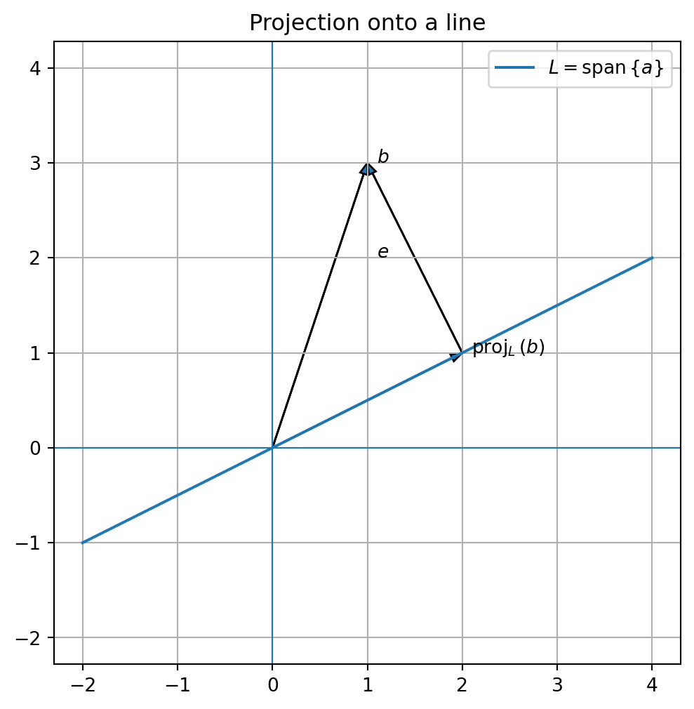
The projection of \(b\) onto the line \(L=\operatorname{span}\{a\}\) is the vector on \(L\) such that the error
\[
e=b-\operatorname{proj}_L(b)
\]
is orthogonal to \(L\) .
Since \(L\) is spanned by \(a\) , this means
\[
a\cdot e=0.
\]
If the projection has the form \(xa\) , then
\[
e=b-xa.
\]
The orthogonality condition becomes
\[
a\cdot(b-xa)=0.
\]
Expanding,
\[
a\cdot b-x(a\cdot a)=0.
\]
Thus
\[
x=\frac{a\cdot b}{a\cdot a}.
\]
Therefore
\[
\operatorname{proj}_L(b)
=
\frac{a\cdot b}{a\cdot a}a.
\]
If \(a\ne 0\) and \(L=\operatorname{span}\{a\}\) , then
\[
\operatorname{proj}_L(b)=\frac{a\cdot b}{a\cdot a}a.
\]
13.3 Example: projection onto a line in \(\mathbb{R}^2\)
Let
\[
a=
\begin{bmatrix}
2\\
1
\end{bmatrix},
\qquad
b=
\begin{bmatrix}
1\\
3
\end{bmatrix}.
\]
Then
\[
a\cdot b=2(1)+1(3)=5,
\]
and
\[
a\cdot a=2^2+1^2=5.
\]
So
\[
\frac{a\cdot b}{a\cdot a}=1.
\]
Therefore
\[
\operatorname{proj}_L(b)=a=
\begin{bmatrix}
2\\
1
\end{bmatrix}.
\]
The error is
\[
e=b-\operatorname{proj}_L(b)
=
\begin{bmatrix}
1\\
3
\end{bmatrix}
-
\begin{bmatrix}
2\\
1
\end{bmatrix}
=
\begin{bmatrix}
-1\\
2
\end{bmatrix}.
\]
Check orthogonality:
\[
a\cdot e=
\begin{bmatrix}
2\\
1
\end{bmatrix}
\cdot
\begin{bmatrix}
-1\\
2
\end{bmatrix}
=
-2+2=0.
\]
13.4 Python plot: projection onto a line
import numpy as npimport matplotlib.pyplot as plt= np.array([2 , 1 ], dtype= float )= np.array([1 , 3 ], dtype= float )= (np.dot(a, b) / np.dot(a, a)) * a= b - proj= np.linspace(- 1 , 2 , 100 )= np.outer(t, a)= (6 , 6 ))0 ], line[:, 1 ], label= "$L= \\ operatorname {span} \\ {a \\ }$" )0 , 0 , b[0 ], b[1 ], head_width= 0.08 , length_includes_head= True )0 , 0 , proj[0 ], proj[1 ], head_width= 0.08 , length_includes_head= True )0 ], proj[1 ], e[0 ], e[1 ], head_width= 0.08 , length_includes_head= True )0 ] + 0.1 , b[1 ], "$b$" )0 ] + 0.1 , proj[1 ], "$ \\ operatorname {proj} _L(b)$" )0 ] + e[0 ]/ 2 - 0.4 , proj[1 ] + e[1 ]/ 2 , "$e$" )0 , linewidth= 0.8 )0 , linewidth= 0.8 )True )"equal" )"Projection onto a line" )
13.5 Parallel plus perpendicular decomposition
Projection gives a decomposition
\[
b=\operatorname{proj}_L(b)+e,
\]
where
\[
\operatorname{proj}_L(b)\in L
\]
and
\[
e\in L^\perp.
\]
That is,
\[
b=b_{\parallel}+b_{\perp}.
\]
Here
\[
b_{\parallel}=\operatorname{proj}_L(b),
\]
and
\[
b_{\perp}=b-\operatorname{proj}_L(b).
\]
This decomposition is one of the central geometric ideas of linear algebra.
Projection decomposes a vector into two perpendicular parts:
\[
b=b_{\parallel}+b_{\perp},
\]
where
\[
b_{\parallel}\in L,
\qquad
b_{\perp}\in L^\perp.
\]
13.6 Projection using a unit vector
If \(q\) is a unit vector, so that
\[
\|q\|=1,
\]
then projection onto the line spanned by \(q\) becomes simpler.
Since
\[
q\cdot q=1,
\]
we get
\[
\operatorname{proj}_{\operatorname{span}\{q\}}(b)=(q\cdot b)q.
\]
If \(\|q\|=1\) , then
\[
\operatorname{proj}_{\operatorname{span}\{q\}}(b)=(q\cdot b)q.
\]
The number \(q\cdot b\) is the coordinate of \(b\) in the \(q\) direction.
13.7 Projection matrix onto a line
Projection onto a line is a linear transformation.
Let
\[
L=\operatorname{span}\{a\}.
\]
Then
\[
\operatorname{proj}_L(b)
=
\frac{a\cdot b}{a\cdot a}a.
\]
Using matrix notation,
\[
a\cdot b=a^Tb.
\]
So
\[
\operatorname{proj}_L(b)
=
a\frac{a^Tb}{a^Ta}
=
\frac{aa^T}{a^Ta}b.
\]
Thus the projection matrix is
\[
P=\frac{aa^T}{a^Ta}.
\]
For \(L=\operatorname{span}\{a\}\) with \(a\ne 0\) ,
\[
P=\frac{aa^T}{a^Ta}.
\]
Then
\[
\operatorname{proj}_L(b)=Pb.
\]
13.8 Example: projection matrix onto a line
Let
\[
a=
\begin{bmatrix}
2\\
1
\end{bmatrix}.
\]
Then
\[
aa^T=
\begin{bmatrix}
2\\
1
\end{bmatrix}
\begin{bmatrix}
2&1
\end{bmatrix}
=
\begin{bmatrix}
4&2\\
2&1
\end{bmatrix}.
\]
Also,
\[
a^Ta=5.
\]
So
\[
P=
\frac{1}{5}
\begin{bmatrix}
4&2\\
2&1
\end{bmatrix}.
\]
For
\[
b=
\begin{bmatrix}
1\\
3
\end{bmatrix},
\]
we get
\[
Pb=
\frac{1}{5}
\begin{bmatrix}
4&2\\
2&1
\end{bmatrix}
\begin{bmatrix}
1\\
3
\end{bmatrix}
=
\frac{1}{5}
\begin{bmatrix}
10\\
5
\end{bmatrix}
=
\begin{bmatrix}
2\\
1
\end{bmatrix}.
\]
This agrees with the projection formula.
13.9 Properties of projection matrices
A projection matrix \(P\) onto a subspace has two key properties.
First,
\[
P^2=P.
\]
Applying the projection twice is the same as applying it once.
Second, for orthogonal projection,
\[
P^T=P.
\]
The matrix is symmetric.
For an orthogonal projection matrix \(P\) ,
\[
P^2=P
\]
and
\[
P^T=P.
\]
The equation \(P^2=P\) is called idempotence .
The equation \(P^T=P\) is symmetry.
13.10 Closest point interpretation
Projection solves a closest point problem.
Let \(L=\operatorname{span}\{a\}\) . Then \(\operatorname{proj}_L(b)\) is the vector in \(L\) closest to \(b\) .
That means
\[
\|b-\operatorname{proj}_L(b)\|
\le
\|b-y\|
\]
for every \(y\in L\) .
Why?
Every \(y\in L\) can be written as
\[
y=\operatorname{proj}_L(b)+z,
\]
where \(z\in L\) .
Then
\[
b-y
=
b-\operatorname{proj}_L(b)-z
=
e-z.
\]
Since \(e\perp L\) and \(z\in L\) , we have \(e\perp z\) .
By the Pythagorean theorem,
\[
\|e-z\|^2=\|e\|^2+\|z\|^2\ge \|e\|^2.
\]
Therefore the closest point occurs when \(z=0\) .
13.11 Projection onto a subspace with an orthonormal basis
Let \(W\) be a subspace with orthonormal basis
\[
q_1,q_2,\ldots,q_k.
\]
Then the projection of \(b\) onto \(W\) is
\[
\operatorname{proj}_W(b)
=
(b\cdot q_1)q_1+(b\cdot q_2)q_2+\cdots+(b\cdot q_k)q_k.
\]
If \(\{q_1,\ldots,q_k\}\) is an orthonormal basis for \(W\) , then
\[
\operatorname{proj}_W(b)=\sum_{j=1}^k (b\cdot q_j)q_j.
\]
This formula is simple because the basis vectors are orthonormal.
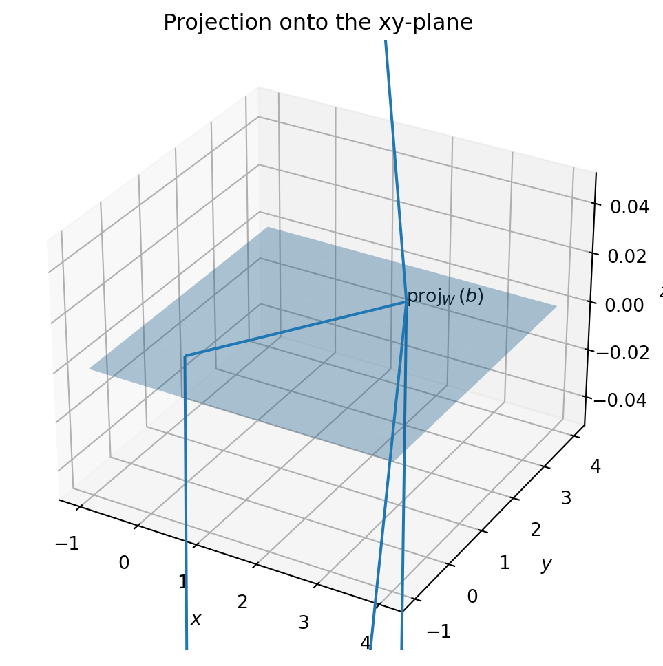
13.13 Example: projection onto a plane in \(\mathbb{R}^3\)
Let
\[
q_1=
\begin{bmatrix}
1\\
0\\
0
\end{bmatrix},
\qquad
q_2=
\begin{bmatrix}
0\\
1\\
0
\end{bmatrix}.
\]
These vectors form an orthonormal basis for the \(xy\) -plane.
For
\[
b=
\begin{bmatrix}
2\\
3\\
5
\end{bmatrix},
\]
the projection onto the \(xy\) -plane is
\[
(b\cdot q_1)q_1+(b\cdot q_2)q_2
=
2
\begin{bmatrix}
1\\
0\\
0
\end{bmatrix}
+
3
\begin{bmatrix}
0\\
1\\
0
\end{bmatrix}
=
\begin{bmatrix}
2\\
3\\
0
\end{bmatrix}.
\]
The error is
\[
e=
\begin{bmatrix}
2\\
3\\
5
\end{bmatrix}
-
\begin{bmatrix}
2\\
3\\
0
\end{bmatrix}
=
\begin{bmatrix}
0\\
0\\
5
\end{bmatrix}.
\]
The error is perpendicular to the \(xy\) -plane.
13.14 Python plot: projection onto the \(xy\) -plane
from mpl_toolkits.mplot3d import Axes3D= np.array([2 , 3 , 5 ], dtype= float )= np.array([2 , 3 , 0 ], dtype= float )= b - proj= np.linspace(- 1 , 4 , 10 )= np.linspace(- 1 , 4 , 10 )= np.meshgrid(x, y)= np.zeros_like(X)= plt.figure(figsize= (7 , 6 ))= fig.add_subplot(111 , projection= "3d" )= 0.35 )0 , 0 , 0 , b[0 ], b[1 ], b[2 ], length= 1 , normalize= False )0 , 0 , 0 , proj[0 ], proj[1 ], proj[2 ], length= 1 , normalize= False )0 ], proj[1 ], proj[2 ], e[0 ], e[1 ], e[2 ], length= 1 , normalize= False )0 ], b[1 ], b[2 ], "$b$" )0 ], proj[1 ], proj[2 ], "$ \\ operatorname {proj} _W(b)$" )"$x$" )"$y$" )"$z$" )"Projection onto the xy-plane" )
13.15 Projection onto a subspace with a nonorthonormal basis
Suppose the columns of \(A\) form a basis for a subspace \(W\) .
If the columns are not orthonormal, then the formula \(AA^T\) does not give the projection.
We need a different formula.
We want to find a vector in \(\operatorname{Col}(A)\) closest to \(b\) .
Every vector in \(\operatorname{Col}(A)\) has the form
\[
Ax.
\]
The error is
\[
e=b-Ax.
\]
At the best approximation, the error must be orthogonal to the column space:
\[
A^T(b-Ax)=0.
\]
Expanding,
\[
A^Tb-A^TAx=0.
\]
So
\[
A^TAx=A^Tb.
\]
These are the normal equations .
To project \(b\) onto \(\operatorname{Col}(A)\) , solve
\[
A^TA\hat x=A^Tb.
\]
Then
\[
\operatorname{proj}_{\operatorname{Col}(A)}(b)=A\hat x.
\]
13.16 Projection matrix for a full-rank matrix
If the columns of \(A\) are linearly independent, then \(A^TA\) is invertible.
The normal equations give
\[
\hat x=(A^TA)^{-1}A^Tb.
\]
Therefore
\[
\operatorname{proj}_{\operatorname{Col}(A)}(b)
=
A(A^TA)^{-1}A^Tb.
\]
So the projection matrix is
\[
P=A(A^TA)^{-1}A^T.
\]
If \(A\) has linearly independent columns, then the orthogonal projection onto \(\operatorname{Col}(A)\) is
\[
P=A(A^TA)^{-1}A^T.
\]
When \(A=Q\) has orthonormal columns,
\[
A^TA=Q^TQ=I,
\]
so the formula becomes
\[
P=QQ^T.
\]
13.17 Example: projection using normal equations
Let
\[
A=
\begin{bmatrix}
1\\
2\\
2
\end{bmatrix},
\qquad
b=
\begin{bmatrix}
2\\
1\\
3
\end{bmatrix}.
\]
Here \(\operatorname{Col}(A)\) is a line in \(\mathbb{R}^3\) .
The normal equation is
\[
A^TA\hat x=A^Tb.
\]
Compute:
\[
A^TA=1^2+2^2+2^2=9,
\]
and
\[
A^Tb=1(2)+2(1)+2(3)=10.
\]
Thus
\[
9\hat x=10,
\]
so
\[
\hat x=\frac{10}{9}.
\]
The projection is
\[
A\hat x=
\frac{10}{9}
\begin{bmatrix}
1\\
2\\
2
\end{bmatrix}
=
\begin{bmatrix}
10/9\\
20/9\\
20/9
\end{bmatrix}.
\]
This agrees with the line projection formula.
13.18 Python: projection using normal equations
= np.array([[1 ],2 ],2 ]], dtype= float )= np.array([2 , 1 , 3 ], dtype= float )= np.linalg.solve(A.T @ A, A.T @ b)= A @ x_hat= b - proj@ error
(array([1.11111111]),
 array([1.11111111, 2.22222222, 2.22222222]),
 array([ 0.88888889, -1.22222222,  0.77777778]),
 array([-4.4408921e-16]))
The last output verifies that the error is orthogonal to the column space.
13.19 Projection and least squares preview
When \(Ax=b\) is inconsistent, there is no exact solution.
But we can still ask for the best approximate solution:
\[
A\hat x \approx b.
\]
The least-squares solution chooses \(\hat x\) to minimize
\[
\|b-Ax\|.
\]
This is exactly a projection problem.
The vector
\[
A\hat x
\]
is the projection of \(b\) onto \(\operatorname{Col}(A)\) .
The error
\[
e=b-A\hat x
\]
is orthogonal to \(\operatorname{Col}(A)\) .
Thus
\[
A^T(b-A\hat x)=0.
\]
So least squares leads to the normal equations:
\[
A^TA\hat x=A^Tb.
\]
We will study least squares more fully in a later chapter.
13.21 Python: projection matrix properties
= np.array([[2 ],1 ]], dtype= float )= a @ a.T / (a.T @ a)@ P, P.T
(array([[0.8, 0.4],
        [0.4, 0.2]]),
 array([[0.8, 0.4],
        [0.4, 0.2]]),
 array([[0.8, 0.4],
        [0.4, 0.2]]))
Check numerically:
@ P, P), np.allclose(P.T, P)
13.22 Algorithmic summary
Given a nonzero vector \(a\) and a vector \(b\) ,
\[
\operatorname{proj}_{\operatorname{span}\{a\}}(b)
=
\frac{a\cdot b}{a\cdot a}a.
\]
If \(\{q_1,\ldots,q_k\}\) is an orthonormal basis for \(W\) , then
\[
\operatorname{proj}_W(b)=\sum_{j=1}^k (b\cdot q_j)q_j.
\]
If \(Q\) has orthonormal columns, then
\[
\operatorname{proj}_{\operatorname{Col}(Q)}(b)=QQ^Tb.
\]
If \(A\) has independent columns, solve
\[
A^TA\hat x=A^Tb.
\]
Then
\[
\operatorname{proj}_{\operatorname{Col}(A)}(b)=A\hat x.
\]
If \(A\) has independent columns, then
\[
P=A(A^TA)^{-1}A^T
\]
is the orthogonal projection matrix onto \(\operatorname{Col}(A)\) .
13.23 Common mistakes
Mistake 1: forgetting that projection depends on a subspace
The expression \(\operatorname{proj}(b)\) is incomplete. We must say what subspace we are projecting onto.
Mistake 2: using \(AA^T\) for nonorthonormal columns
The formula
\[
P=QQ^T
\]
works when \(Q\) has orthonormal columns.
For general independent columns \(A\) , use
\[
P=A(A^TA)^{-1}A^T.
\]
Mistake 3: thinking the error is zero
The projection error is zero only if \(b\) already lies in the subspace.
Mistake 4: forgetting the error is orthogonal
For orthogonal projection,
\[
b-\operatorname{proj}_W(b)
\]
is orthogonal to \(W\) .
13.24 Chapter summary
Projection finds the closest vector in a subspace.
For a line \(L=\operatorname{span}\{a\}\) ,
\[
\operatorname{proj}_L(b)=\frac{a\cdot b}{a\cdot a}a.
\]
Projection decomposes a vector as
\[
b=b_{\parallel}+b_{\perp},
\]
where
\[
b_{\parallel}\in L
\]
and
\[
b_{\perp}\in L^\perp.
\]
If \(Q\) has orthonormal columns, then the projection onto \(\operatorname{Col}(Q)\) is
\[
QQ^Tb.
\]
If \(A\) has independent columns, then the projection onto \(\operatorname{Col}(A)\) is
\[
A(A^TA)^{-1}A^Tb.
\]
The normal equations are
\[
A^TA\hat x=A^Tb.
\]
Projection matrices satisfy
\[
P^2=P
\]
and, for orthogonal projections,
\[
P^T=P.
\]
Projection is the geometric foundation of least squares, regression, QR factorization, PCA, and the SVD.
Exercises
A. Projection onto a line
For each pair \(a,b\) , compute \(\operatorname{proj}_{\operatorname{span}\{a\}}(b)\) and the error \(e=b-\operatorname{proj}(b)\) .
\[
a=\begin{bmatrix}2\\1\end{bmatrix},
\qquad
b=\begin{bmatrix}1\\3\end{bmatrix}.
\]
\[
a=\begin{bmatrix}1\\1\end{bmatrix},
\qquad
b=\begin{bmatrix}4\\2\end{bmatrix}.
\]
\[
a=\begin{bmatrix}1\\2\\2\end{bmatrix},
\qquad
b=\begin{bmatrix}2\\1\\3\end{bmatrix}.
\]
\[
a=\begin{bmatrix}3\\0\\4\end{bmatrix},
\qquad
b=\begin{bmatrix}1\\2\\1\end{bmatrix}.
\]
B. Projection matrices
For each vector \(a\) , compute the projection matrix onto \(\operatorname{span}\{a\}\) .
\[
a=\begin{bmatrix}1\\0\end{bmatrix}
\]
\[
a=\begin{bmatrix}0\\1\end{bmatrix}
\]
\[
a=\begin{bmatrix}2\\1\end{bmatrix}
\]
\[
a=\begin{bmatrix}1\\1\\1\end{bmatrix}
\]
For each matrix \(P\) , verify that \(P^2=P\) and \(P^T=P\) .
C. Projection with orthonormal bases
Let
\[
q_1=
\begin{bmatrix}
1\\0\\0
\end{bmatrix},
\qquad
q_2=
\begin{bmatrix}
0\\1\\0
\end{bmatrix}.
\]
Project
\[
b=\begin{bmatrix}2\\3\\5\end{bmatrix}
\]
onto \(\operatorname{span}\{q_1,q_2\}\) .
Find the error vector.
Verify that the error is orthogonal to both \(q_1\) and \(q_2\) .
D. Normal equations
For each matrix \(A\) and vector \(b\) , solve the normal equations and find the projection of \(b\) onto \(\operatorname{Col}(A)\) .
\[
A=
\begin{bmatrix}
1\\2\\2
\end{bmatrix},
\qquad
b=
\begin{bmatrix}
2\\1\\3
\end{bmatrix}.
\]
\[
A=
\begin{bmatrix}
1&0\\
0&1\\
1&1
\end{bmatrix},
\qquad
b=
\begin{bmatrix}
2\\1\\4
\end{bmatrix}.
\]
\[
A=
\begin{bmatrix}
1&1\\
1&2\\
1&3
\end{bmatrix},
\qquad
b=
\begin{bmatrix}
1\\2\\2
\end{bmatrix}.
\]
E. Closest point interpretation
Explain why the projection is the closest point in a subspace.
Explain why the projection error must be orthogonal to the subspace.
Use the Pythagorean theorem to justify the closest point property.
F. Python exercises
Write a Python function that computes projection onto a line.
Plot \(b\) , \(\operatorname{proj}_L(b)\) , and the error vector for a line in \(\mathbb{R}^2\) .
Compute a projection matrix \(P\) and verify \(P^2=P\) and \(P^T=P\) .
Use normal equations to project a vector onto the column space of a matrix.
Plot a projection onto the \(xy\) -plane in \(\mathbb{R}^3\) .
G. Reflection
Write a short paragraph answering each question.
Why is projection a closest point problem?
Why is the projection error orthogonal to the subspace?
Why does an orthonormal basis make projection easier?
Why do normal equations appear in projection?
How does projection prepare for least squares?
AI-age connection
Projection is one of the central operations in computational data analysis. Least squares regression projects observed data onto a model space. Dimensionality reduction projects high-dimensional data onto lower-dimensional structures. PCA finds the best projection directions for preserving variance. Neural-network embeddings and feature maps often rely on geometric notions of similarity, distance, and approximation. Projection is the mathematical language of optimal linear approximation.