Opening question
In Chapter 10, we learned that a matrix represents a linear transformation:
\[
T(x)=Ax.
\]
But in applications, transformations rarely occur alone. We often apply one process after another:
scale a vector,
rotate it,
project it,
change coordinates,
apply a model,
transform the output again.
What matrix represents the combined process?
The answer is matrix multiplication.
If
\[
T(x)=Bx
\]
and
\[
S(y)=Ay,
\]
then applying \(T\) first and then \(S\) gives
\[
S(T(x))=A(Bx)=(AB)x.
\]
Thus:
Matrix multiplication is composition of linear transformations.
This chapter develops composition, inverse transformations, geometric transformations, and the meaning of matrix products as chained linear processes.
Learning goals
After studying this chapter, you should be able to:
Define composition of functions.
Interpret matrix multiplication as composition of linear transformations.
Determine the correct order of matrix products.
Compute standard matrices for composed transformations.
Understand why matrix multiplication is usually not commutative.
Use inverses to reverse linear transformations.
Interpret inverse matrices as inverse transformations.
Analyze rotations, reflections, projections, shears, and scalings.
Visualize compositions using Python plots.
Connect composition to computational pipelines and AI models.
11.1 Composition of functions
If
\[
T:\mathbb{R}^n\to\mathbb{R}^m
\]
and
\[
S:\mathbb{R}^m\to\mathbb{R}^p,
\]
then the composition
\[
S\circ T:\mathbb{R}^n\to\mathbb{R}^p
\]
is defined by
\[
(S\circ T)(x)=S(T(x)).
\]
This means:
first apply \(T\) to \(x\) ,
then apply \(S\) to the result.
The order matters. The notation \(S\circ T\) means \(T\) acts first.
11.3 Order matters
The product
\[
ABx
\]
means
\[
A(Bx).
\]
So \(B\) acts first and \(A\) acts second.
This is often the opposite of how we read from left to right. For transformations, read from right to left:
\[
ABx
=
\text{first }B,\text{ then }A.
\]
For example, if
\[
B
\]
is a rotation and
\[
A
\]
is a projection, then
\[
AB
\]
means:
rotate,
then project.
But
\[
BA
\]
means:
project,
then rotate.
These usually produce different results.
11.4 Example: rotation followed by projection
Let
\[
R=
\begin{bmatrix}
0&-1\\
1&0
\end{bmatrix}
\]
be rotation by \(90^\circ\) counterclockwise, and let
\[
P=
\begin{bmatrix}
1&0\\
0&0
\end{bmatrix}
\]
be projection onto the \(x\) -axis.
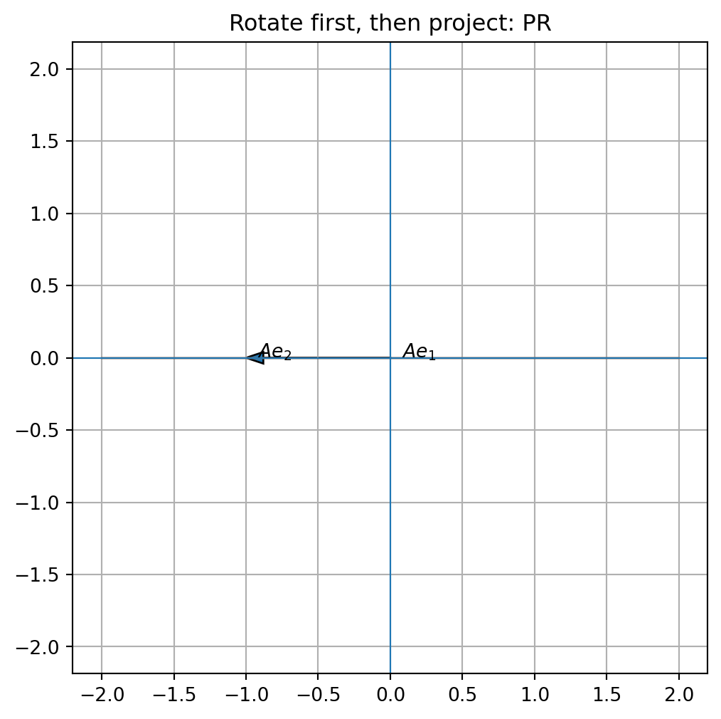
The composition “rotate first, then project” has matrix
\[
PR.
\]
Compute:
\[
PR=
\begin{bmatrix}
1&0\\
0&0
\end{bmatrix}
\begin{bmatrix}
0&-1\\
1&0
\end{bmatrix}
=
\begin{bmatrix}
0&-1\\
0&0
\end{bmatrix}.
\]
Therefore
\[
PR
\begin{bmatrix}
x\\y
\end{bmatrix}
=
\begin{bmatrix}
-y\\
0
\end{bmatrix}.
\]
11.5 Example: projection followed by rotation
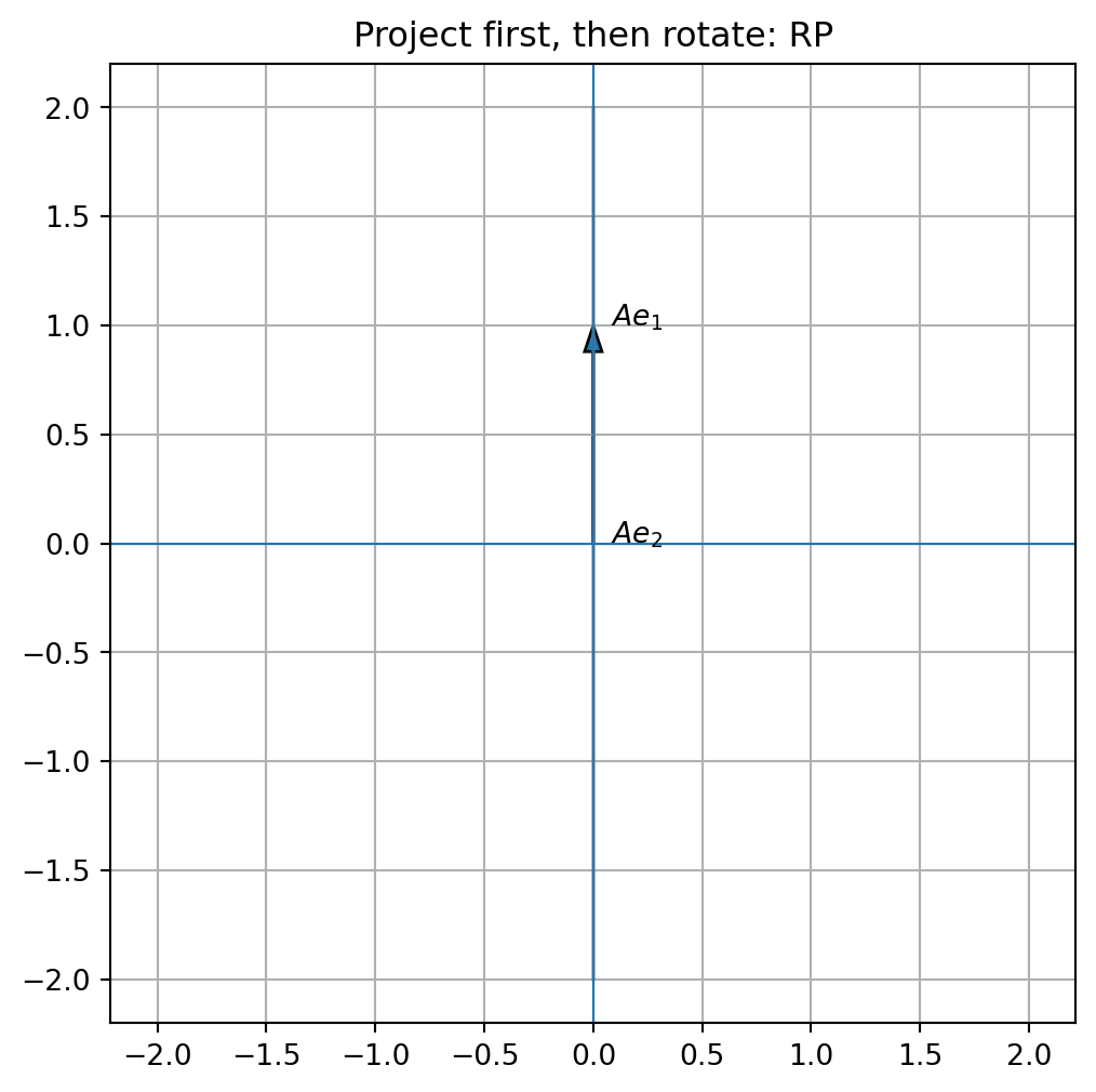
Now apply projection first and then rotation. The matrix is
\[
RP.
\]
Compute:
\[
RP=
\begin{bmatrix}
0&-1\\
1&0
\end{bmatrix}
\begin{bmatrix}
1&0\\
0&0
\end{bmatrix}
=
\begin{bmatrix}
0&0\\
1&0
\end{bmatrix}.
\]
Thus
\[
RP
\begin{bmatrix}
x\\y
\end{bmatrix}
=
\begin{bmatrix}
0\\
x
\end{bmatrix}.
\]
Since
\[
PR\ne RP,
\]
the order matters.
This is a geometric explanation for why matrix multiplication is usually not commutative.
11.6 Python visualization: composition order
import numpy as npimport matplotlib.pyplot as pltdef plot_transformed_grid(A, title):= np.linspace(- 2 , 2 , 9 )= np.linspace(- 2 , 2 , 9 )= (6 , 6 ))for x in xs:= np.array([[x, y] for y in ys])= pts @ A.T0 ], trans[:, 1 ], linewidth= 0.8 )for y in ys:= np.array([[x, y] for x in xs])= pts @ A.T0 ], trans[:, 1 ], linewidth= 0.8 )= A @ np.array([1 , 0 ])= A @ np.array([0 , 1 ])0 , 0 , e1[0 ], e1[1 ], head_width= 0.08 , length_includes_head= True )0 , 0 , e2[0 ], e2[1 ], head_width= 0.08 , length_includes_head= True )0 ] + 0.08 , e1[1 ], "$Ae_1$" )0 ] + 0.08 , e2[1 ], "$Ae_2$" )0 , linewidth= 0.8 )0 , linewidth= 0.8 )True )"equal" )= np.array([[0 , - 1 ],1 , 0 ]], dtype= float )= np.array([[1 , 0 ],0 , 0 ]], dtype= float )@ R, "Rotate first, then project: PR" )@ P, "Project first, then rotate: RP" )
The two plots show different collapsed lines. This is composition order made visible.
11.7 Composition preserves linearity
If
\[
T:\mathbb{R}^n\to\mathbb{R}^m
\]
and
\[
S:\mathbb{R}^m\to\mathbb{R}^p
\]
are linear transformations, then
\[
S\circ T
\]
is also linear.
Indeed,
\[
(S\circ T)(u+v)=S(T(u+v)).
\]
Since \(T\) is linear,
\[
T(u+v)=T(u)+T(v).
\]
So
\[
S(T(u+v))=S(T(u)+T(v)).
\]
Since \(S\) is linear,
\[
S(T(u)+T(v))=S(T(u))+S(T(v)).
\]
Therefore
\[
(S\circ T)(u+v)=(S\circ T)(u)+(S\circ T)(v).
\]
Similarly,
\[
(S\circ T)(cu)=c(S\circ T)(u).
\]
Thus the composition is linear.
11.10 Rotation matrices
The rotation matrix
\[
R_\theta=
\begin{bmatrix}
\cos\theta&-\sin\theta\\
\sin\theta&\cos\theta
\end{bmatrix}
\]
rotates every vector counterclockwise by angle \(\theta\) .
Important special cases:
For \(\theta=0\) ,
\[
R_0=I.
\]
For \(\theta=\frac{\pi}{2}\) ,
\[
R_{\pi/2}=
\begin{bmatrix}
0&-1\\
1&0
\end{bmatrix}.
\]
For \(\theta=\pi\) ,
\[
R_{\pi}=
\begin{bmatrix}
-1&0\\
0&-1
\end{bmatrix}.
\]
Rotation matrices satisfy
\[
R_\alpha R_\beta=R_{\alpha+\beta}.
\]
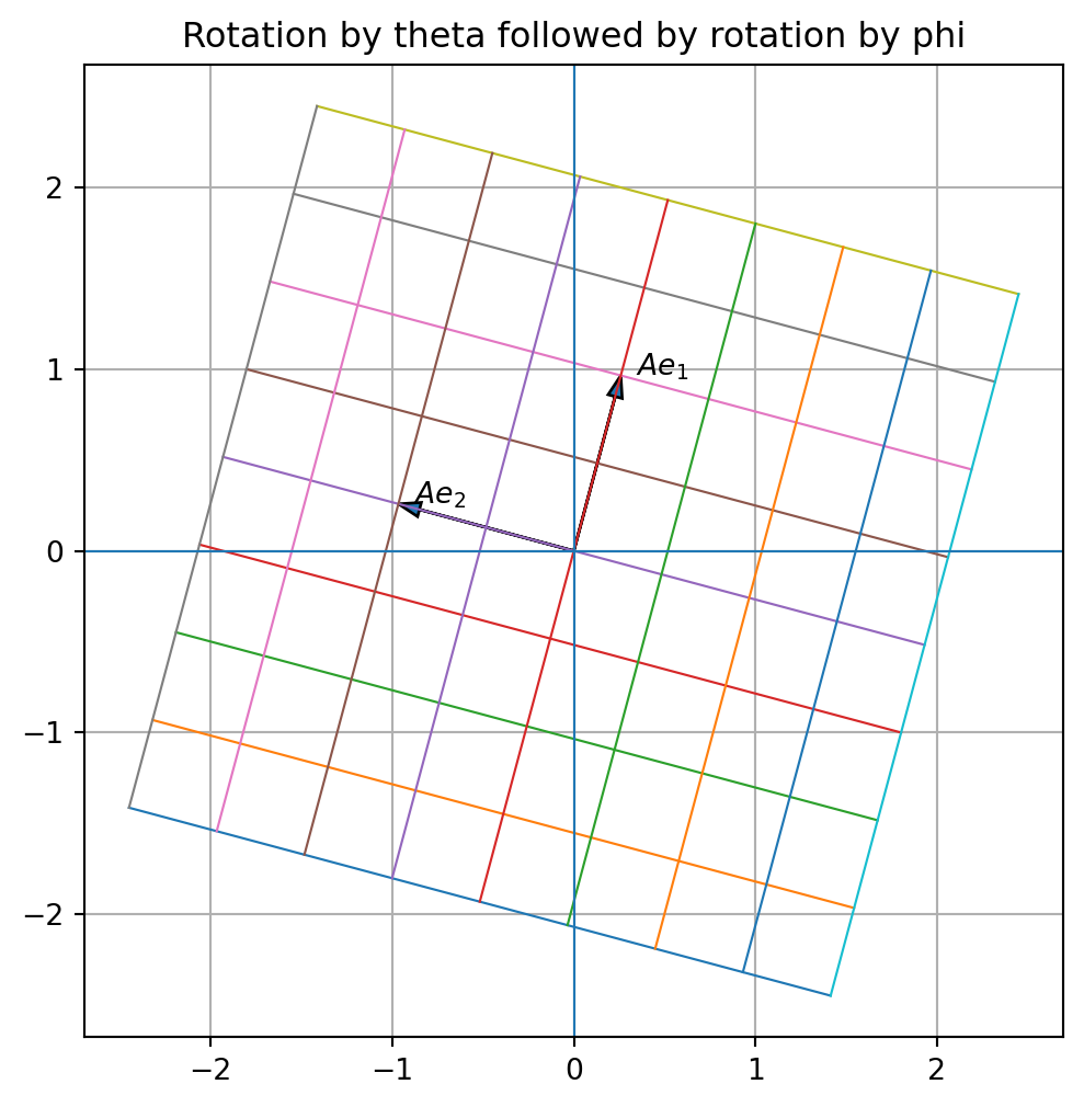
This means composing rotations adds angles.
11.11 Python visualization: composing rotations
= np.pi / 6 = np.pi / 4 = np.array([- np.sin(theta)],= np.array([- np.sin(phi)],= R_phi @ R_theta= np.array([+ phi), - np.sin(theta + phi)],+ phi), np.cos(theta + phi)]
(array([[ 0.25881905, -0.96592583],
        [ 0.96592583,  0.25881905]]),
 array([[ 0.25881905, -0.96592583],
        [ 0.96592583,  0.25881905]]))
The two matrices are the same up to roundoff error.
"Rotation by theta followed by rotation by phi" )
11.12 Shears and scalings
A horizontal shear
\[
H_k=
\begin{bmatrix}
1&k\\
0&1
\end{bmatrix}
\]
maps
\[
(x,y)\mapsto (x+ky,y).
\]
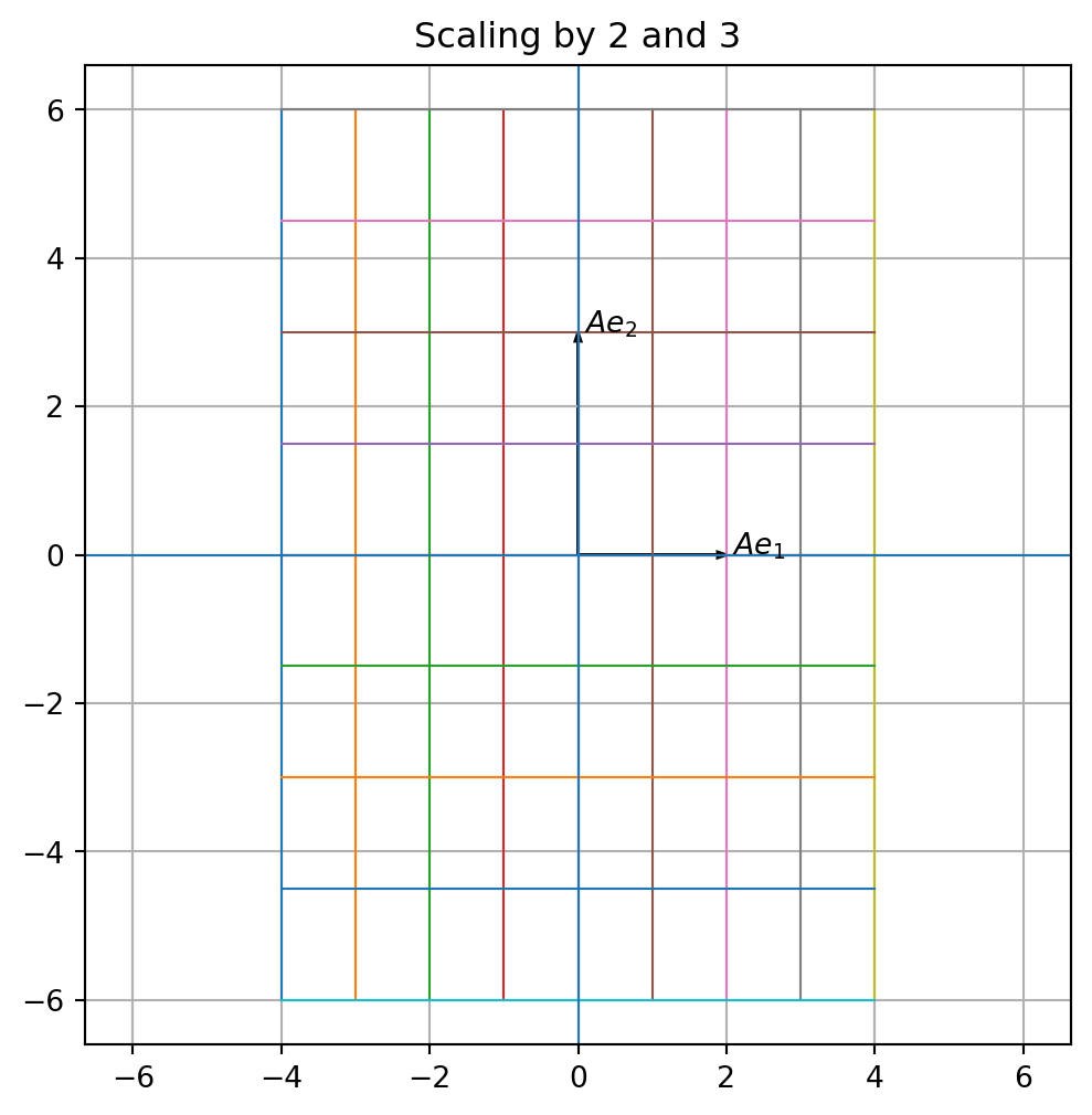
A scaling
\[
S=
\begin{bmatrix}
a&0\\
0&b
\end{bmatrix}
\]
maps
\[
(x,y)\mapsto (ax,by).
\]
The compositions
\[
SH_k
\]
and
\[
H_kS
\]
are generally different.
Compute \(SH_k\)
\[
SH_k=
\begin{bmatrix}
a&0\\
0&b
\end{bmatrix}
\begin{bmatrix}
1&k\\
0&1
\end{bmatrix}
=
\begin{bmatrix}
a&ak\\
0&b
\end{bmatrix}.
\]
Compute \(H_kS\)
\[
H_kS=
\begin{bmatrix}
1&k\\
0&1
\end{bmatrix}
\begin{bmatrix}
a&0\\
0&b
\end{bmatrix}
=
\begin{bmatrix}
a&kb\\
0&b
\end{bmatrix}.
\]
These are equal only when
\[
ak=kb.
\]
If \(k\ne 0\) , this means \(a=b\) .
So scaling and shearing usually do not commute.
11.15 Inverse of a composition
If \(A\) and \(B\) are invertible, then \(AB\) is invertible and
\[
(AB)^{-1}=B^{-1}A^{-1}.
\]
The order reverses.
Why?
The product \(AB\) means first apply \(B\) , then apply \(A\) .
To undo this process, we must first undo \(A\) , then undo \(B\) .
So the inverse is
\[
B^{-1}A^{-1}.
\]
Check:
\[
(AB)(B^{-1}A^{-1})
=
A(BB^{-1})A^{-1}
=
AIA^{-1}
=
AA^{-1}
=
I.
\]
Similarly,
\[
(B^{-1}A^{-1})(AB)=I.
\]
If \(A\) and \(B\) are invertible, then
\[
(AB)^{-1}=B^{-1}A^{-1}.
\]
11.17 Composition and coordinate change
Change of basis is also a composition.
Suppose \(A\) is a matrix in standard coordinates and \(P\) is a basis matrix.
The matrix in the new basis is
\[
P^{-1}AP.
\]
This product means:
start with coordinates in the new basis,
multiply by \(P\) to convert to standard coordinates,
apply \(A\) in standard coordinates,
multiply by \(P^{-1}\) to convert back to the new basis.
So
\[
P^{-1}AP
\]
is a composition of three transformations.
This is the conceptual meaning of similarity.
11.18 Computational pipelines
A computational pipeline often has the form
\[
x\mapsto A_1x\mapsto A_2A_1x\mapsto A_3A_2A_1x.
\]
Examples:
preprocess data,
rotate or project features,
apply a model matrix,
transform the output.
The combined linear part of the pipeline is a matrix product.
In neural networks, a purely linear sequence of layers without nonlinear activation would collapse into a single matrix product:
\[
A_kA_{k-1}\cdots A_1x.
\]
This is why nonlinear activation functions are essential in deep learning. Without nonlinearities, many linear layers are just one linear layer.
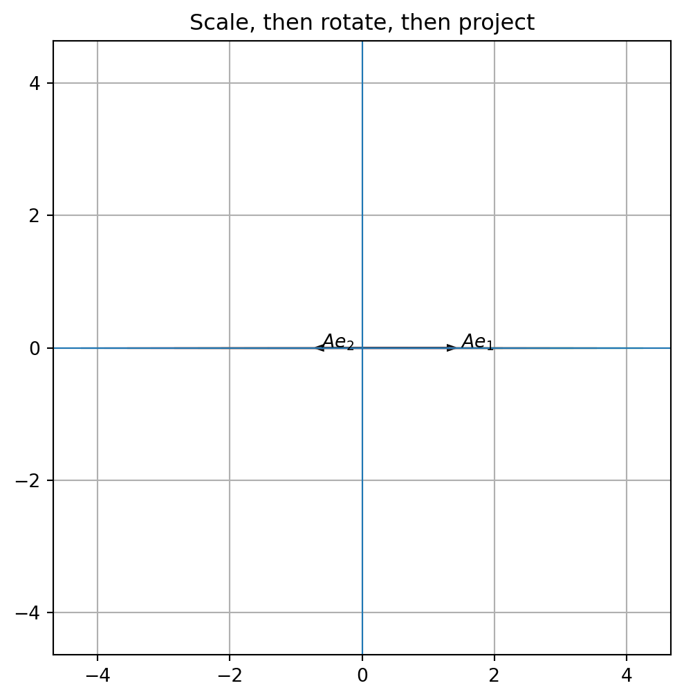
11.19 Python: a simple linear pipeline
# Step 1: scale = np.array([[2 , 0 ],0 , 1 ]], dtype= float )# Step 2: rotate = np.pi / 4 = np.array([- np.sin(theta)],# Step 3: project = np.array([[1 , 0 ],0 , 0 ]], dtype= float )# Combined transformation: scale first, then rotate, then project = P @ R @ S"Scale, then rotate, then project" )
The combined matrix is
\[
A_{\text{total}}=PRS.
\]
The rightmost matrix \(S\) acts first.
11.20 Algorithmic summary
Suppose
\[
T_1(x)=A_1x,\quad T_2(x)=A_2x,\quad \ldots,\quad T_k(x)=A_kx.
\]
If we apply \(T_1\) first, then \(T_2\) , and continue until \(T_k\) , then the combined matrix is
\[
A_kA_{k-1}\cdots A_1.
\]
If \(T(x)=Ax\) and \(A\) is invertible, then
\[
T^{-1}(x)=A^{-1}x.
\]
If \(A\) is not invertible, then \(T\) has no inverse transformation.
If \(A_1,\ldots,A_k\) are invertible, then
\[
(A_kA_{k-1}\cdots A_1)^{-1}
=
A_1^{-1}\cdots A_{k-1}^{-1}A_k^{-1}.
\]
The inverse order reverses.
11.21 Common mistakes
Mistake 2: assuming \(AB=BA\)
Compositions usually depend on order, so matrix multiplication is usually not commutative.
Mistake 4: trying to invert a projection
Projection loses information and does not have an inverse transformation.
Mistake 5: forgetting dimension compatibility
For \(S\circ T\) to be defined, the output space of \(T\) must match the input space of \(S\) .
For matrix products, the inner dimensions must match.
11.22 Chapter summary
Composition means applying one transformation after another.
If
\[
T(x)=Bx
\]
and
\[
S(y)=Ay,
\]
then
\[
(S\circ T)(x)=A(Bx)=(AB)x.
\]
So the matrix of the composition is
\[
AB.
\]
The rightmost matrix acts first.
Matrix multiplication is usually not commutative because transformation order usually matters.
A linear transformation \(T(x)=Ax\) is invertible exactly when \(A\) is invertible.
In that case,
\[
T^{-1}(x)=A^{-1}x.
\]
If \(A\) and \(B\) are invertible, then
\[
(AB)^{-1}=B^{-1}A^{-1}.
\]
Change of basis is a composition:
\[
P^{-1}AP.
\]
A linear computational pipeline can be represented as a product of matrices.
Exercises
A. Composition order
Let
\[
R=
\begin{bmatrix}
0&-1\\
1&0
\end{bmatrix},
\qquad
P=
\begin{bmatrix}
1&0\\
0&0
\end{bmatrix}.
\]
Compute \(PR\) .
Compute \(RP\) .
Apply both matrices to
\[
x=
\begin{bmatrix}
2\\
3
\end{bmatrix}.
\]
Explain geometrically why the results are different.
D. Inverse of a product
Let
\[
A=
\begin{bmatrix}
1&1\\
0&1
\end{bmatrix},
\qquad
B=
\begin{bmatrix}
2&0\\
0&3
\end{bmatrix}.
\]
Compute \(AB\) .
Compute \((AB)^{-1}\) directly.
Compute \(B^{-1}A^{-1}\) .
Verify that the answers in parts 2 and 3 agree.
E. Change of basis as composition
Let
\[
A=
\begin{bmatrix}
2&1\\
0&3
\end{bmatrix}
\]
and
\[
P=
\begin{bmatrix}
1&1\\
1&-1
\end{bmatrix}.
\]
Explain the steps represented by \(P^{-1}AP\) .
Compute \(P^{-1}AP\) .
Interpret the result as the matrix of the same transformation in a new basis.
F. Python exercises
Write a Python function to plot the image of a grid under a \(2\times 2\) matrix.
Plot \(PR\) and \(RP\) for projection and rotation.
Plot a composition of scaling, rotation, and projection.
Verify numerically that \((AB)^{-1}=B^{-1}A^{-1}\) for two invertible matrices.
Find two matrices \(A\) and \(B\) such that \(AB\ne BA\) , and visualize the two transformations.
G. Reflection
Write a short paragraph answering each question.
Why does matrix multiplication represent composition?
Why does the rightmost matrix act first?
Why is matrix multiplication usually not commutative?
Why does the inverse of a product reverse order?
How does composition appear in computational pipelines?
AI-age connection
Modern computational models are built from composed transformations. Data preprocessing, feature maps, projections, linear layers, and coordinate changes can all be represented by matrices when they are linear. A sequence of linear transformations collapses into one matrix product. This is why nonlinear operations are essential in deep learning: without nonlinearities, many layers would simply be one linear transformation. Composition is therefore the bridge from matrix algebra to computational pipelines.