Opening question
Linear algebra began in this book with systems of equations.
Then matrices became transformations.
Vectors became data points.
Subspaces became model spaces.
Orthogonality became geometry.
Eigenvectors and singular vectors became hidden directions.
Now we bring these ideas together.
Modern data science and artificial intelligence are built on linear algebra. Data sets are matrices. Images are arrays. Text is represented by vectors. Similarity is measured by dot products. Models use matrix multiplication. Least squares fits parameters. PCA and the SVD find low-dimensional structure. Neural networks are built from linear maps and nonlinear activations.
The central question of this final chapter is:
How do the ideas of linear algebra become the language of data and AI?
This chapter is a synthesis. It reviews the key ideas of the course through modern computational examples.
Learning goals
After studying this chapter, you should be able to:
Represent data sets as matrices.
Interpret rows and columns of a data matrix.
Use dot products, norms, and cosine similarity to compare data.
Understand linear models as matrix equations.
Use least squares for prediction.
Explain PCA using eigenvectors and the SVD.
Understand low-rank approximation as compression and denoising.
Interpret neural-network layers as affine transformations followed by nonlinearities.
Use matrices to represent graphs and networks.
See linear algebra as the common language behind data, computation, and AI.
22.1 Data as a matrix
A data set with \(m\) observations and \(n\) features can be represented as a matrix
\[
X=
\begin{bmatrix}
--- x_1^T ---\\
--- x_2^T ---\\
\vdots\\
--- x_m^T ---
\end{bmatrix}.
\]
Here each row
\[
x_i^T
\]
is one observation, and each column is one feature.
For example, if we measure height, weight, and age for \(m\) people, then
\[
X=
\begin{bmatrix}
\text{height}_1&\text{weight}_1&\text{age}_1\\
\text{height}_2&\text{weight}_2&\text{age}_2\\
\vdots&\vdots&\vdots\\
\text{height}_m&\text{weight}_m&\text{age}_m
\end{bmatrix}.
\]
Thus a data set is not only a table. It is a collection of vectors in \(\mathbb{R}^n\) .
Each data point is a point in feature space.
22.2 Rows, columns, and meaning
The two viewpoints of a data matrix are both important.
Row viewpoint
Rows are data points.
Each row vector
\[
x_i\in\mathbb{R}^n
\]
describes one observation using \(n\) features.
This viewpoint supports:
clustering,
nearest neighbors,
classification,
visualization,
embeddings,
similarity search.
Column viewpoint
Columns are features.
Each column vector records one variable across all observations.
This viewpoint supports:
correlation,
regression,
feature selection,
covariance,
PCA,
linear models.
Linear algebra lets us move between these viewpoints.
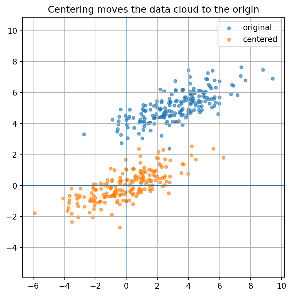
22.3 Centering and scaling data
Before analyzing data, we often center each feature by subtracting its mean.
If \(X\) is a data matrix, the centered data matrix is
\[
X_c=X-\mathbf{1}\mu^T,
\]
where \(\mu\) is the vector of column means.
Centering makes each feature have mean zero.
We may also scale each feature by its standard deviation, giving standardized data.
Centering and scaling are linear-algebraic preprocessing steps.
They change the coordinate system in which data geometry is measured.
22.4 Python: data matrix, centering, and scaling
import numpy as npimport matplotlib.pyplot as plt= np.random.default_rng(0 )# Synthetic data with two features = rng.multivariate_normal(= [3 , 5 ],= [[4 , 1.5 ], [1.5 , 1 ]],= 200 = X.mean(axis= 0 )= X - mu= X_centered.std(axis= 0 , ddof= 1 )= X_centered / std
(array([3.18878164, 5.09467867]), array([1.97691788, 0.9654219 ]))
= (6 , 6 ))0 ], X[:, 1 ], s= 15 , alpha= 0.6 , label= "original" )0 ], X_centered[:, 1 ], s= 15 , alpha= 0.6 , label= "centered" )0 , linewidth= 0.8 )0 , linewidth= 0.8 )True )"equal" )"Centering moves the data cloud to the origin" )
22.5 Dot products and similarity
The dot product measures alignment.
For vectors \(x,y\in\mathbb{R}^n\) ,
\[
x\cdot y=x^Ty.
\]
If \(x\cdot y\) is large and positive, the vectors point in similar directions.
If \(x\cdot y=0\) , the vectors are orthogonal.
If \(x\cdot y\) is negative, the vectors point in opposing directions.
In data science, dot products appear in:
linear prediction,
similarity search,
embeddings,
attention mechanisms,
kernel methods,
recommendation systems.
22.6 Cosine similarity
When magnitude is less important than direction, we use cosine similarity:
\[
\operatorname{cosine}(x,y)
=
\frac{x\cdot y}{\|x\|\|y\|}.
\]
This is the cosine of the angle between the vectors.
Cosine similarity lies between \(-1\) and \(1\) .
\(1\) means same direction,\(0\) means orthogonal,\(-1\) means opposite directions.
For nonzero vectors \(x\) and \(y\) ,
\[
\operatorname{cosine}(x,y)
=
\frac{x^Ty}{\|x\|\|y\|}.
\]
22.7 Python: cosine similarity
def cosine_similarity(x, y):return np.dot(x, y) / (np.linalg.norm(x) * np.linalg.norm(y))= np.array([1 , 2 , 3 ], dtype= float )= np.array([2 , 4 , 6 ], dtype= float )= np.array([3 , - 2 , 1 ], dtype= float )
(1.0, 0.14285714285714285)
The first value is \(1\) because \(y=2x\) .
The second value is closer to \(0\) because \(z\) is less aligned with \(x\) .
22.8 Linear prediction
A linear model predicts an output using a dot product.
For a feature vector
\[
x=
\begin{bmatrix}
x_1\\
\vdots\\
x_n
\end{bmatrix},
\]
a linear prediction has the form
\[
\hat y=w^Tx+b.
\]
Here:
\(w\) is a vector of weights,\(b\) is an intercept,\(\hat y\) is the predicted value.
If we include a constant feature \(1\) , then we can write the model as one dot product:
\[
\hat y=\beta^T\tilde x,
\]
where
\[
\tilde x=
\begin{bmatrix}
1\\
x_1\\
\vdots\\
x_n
\end{bmatrix},
\qquad
\beta=
\begin{bmatrix}
b\\
w_1\\
\vdots\\
w_n
\end{bmatrix}.
\]
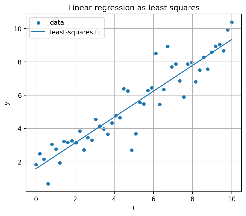
22.9 Linear regression as least squares
For many observations, the linear model becomes
\[
A\beta\approx y.
\]
The least-squares solution minimizes
\[
\|y-A\beta\|^2.
\]
The normal equations are
\[
A^TA\hat\beta=A^Ty.
\]
Computationally, we usually use QR or SVD rather than explicitly forming \(A^TA\) .
Linear regression is the basic example of learning from data by minimizing error.
22.10 Python: linear regression from matrices
= np.random.default_rng(1 )= np.linspace(0 , 10 , 50 )= 1.5 + 0.8 * t + rng.normal(scale= 1.0 , size= len (t))= np.column_stack([np.ones_like(t), t])= np.linalg.lstsq(A, y, rcond= None )[0 ]= A @ beta= (6 , 5 ))= 20 , label= "data" )= "least-squares fit" )"$t$" )"$y$" )True )"Linear regression as least squares" )
array([1.58556853, 0.77567068])
The fitted line is
\[
\hat y=\hat\beta_0+\hat\beta_1t.
\]
22.11 Feature maps
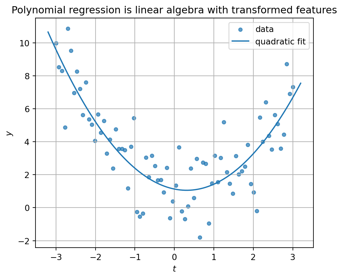
A model may be nonlinear in the original input but linear in transformed features.
For example, polynomial regression uses features
\[
1,\ t,\ t^2,\ldots,t^d.
\]
The model
\[
\hat y=\beta_0+\beta_1t+\beta_2t^2
\]
is nonlinear in \(t\) but linear in the parameters \(\beta\) .
The design matrix is
\[
A=
\begin{bmatrix}
1&t_1&t_1^2\\
1&t_2&t_2^2\\
\vdots&\vdots&\vdots\\
1&t_m&t_m^2
\end{bmatrix}.
\]
Feature engineering often means choosing a useful vector representation of data.
Once data is represented as vectors, linear algebra can be applied.
22.12 Python: polynomial features
= np.random.default_rng(2 )= np.linspace(- 3 , 3 , 80 )= 1 - 0.5 * t + 0.8 * t** 2 + rng.normal(scale= 1.5 , size= len (t))= np.column_stack([np.ones_like(t), t, t** 2 ])= np.linalg.lstsq(A, y, rcond= None )[0 ]= np.linspace(- 3.2 , 3.2 , 200 )= np.column_stack([np.ones_like(t_grid), t_grid, t_grid** 2 ])= A_grid @ beta= (6 , 5 ))= 18 , alpha= 0.7 , label= "data" )= "quadratic fit" )"$t$" )"$y$" )True )"Polynomial regression is linear algebra with transformed features" )
array([ 1.13020673, -0.48494825, 0.77831217])
22.13 Dimensionality reduction
High-dimensional data often contains lower-dimensional structure.
For example, data in \(\mathbb{R}^{1000}\) may approximately lie near a low-dimensional subspace.
Dimensionality reduction seeks a simpler representation:
\[
\mathbb{R}^n \to \mathbb{R}^k,
\qquad
k<n.
\]
Linear dimensionality reduction means projecting data onto a lower-dimensional subspace.
The most important linear method is PCA.
PCA finds directions that preserve as much variance as possible.
22.14 PCA through covariance
Let \(X_c\) be a centered data matrix.
The covariance matrix is
\[
C=\frac{1}{m-1}X_c^TX_c.
\]
This matrix is symmetric positive semidefinite.
Its eigenvectors give principal directions.
Its eigenvalues give variance along those directions.
If
\[
Cv_i=\lambda_i v_i,
\]
then \(v_i\) is a principal component direction and \(\lambda_i\) is the variance explained in that direction.
22.15 PCA through SVD
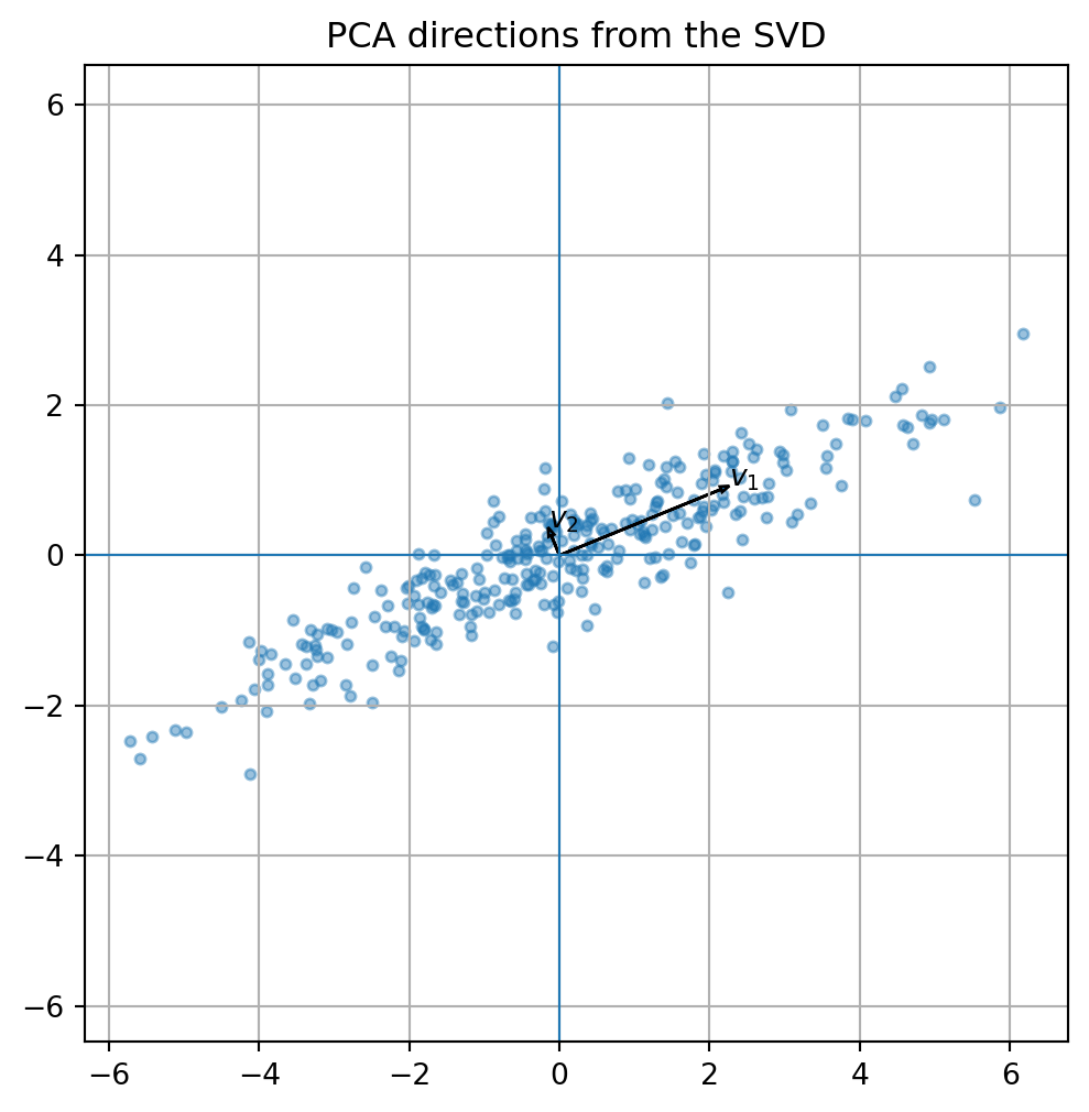
PCA can also be computed using the SVD.
Let
\[
X_c=U\Sigma V^T.
\]
Then
\[
X_c^TX_c=V\Sigma^T\Sigma V^T.
\]
Therefore the right singular vectors in \(V\) are eigenvectors of the covariance matrix.
The variances are
\[
\frac{\sigma_i^2}{m-1}.
\]
Thus PCA is an SVD of the centered data matrix.
For centered data \(X_c\) , the principal component directions are the right singular vectors of \(X_c\) .
22.16 Python: PCA by SVD
= np.random.default_rng(3 )= rng.multivariate_normal(= [0 , 0 ],= [[5 , 2 ], [2 , 1 ]],= 300 = X - X.mean(axis= 0 )= np.linalg.svd(Xc, full_matrices= False )= Vt.T= s** 2 / (len (Xc) - 1 )= (6 , 6 ))0 ], Xc[:, 1 ], s= 12 , alpha= 0.45 )for j in range (2 ):= V[:, j]= np.sqrt(explained_variance[j])0 , 0 , length* direction[0 ], length* direction[1 ],= 0.08 , length_includes_head= True )* direction[0 ], length* direction[1 ], f"$v_ { j+ 1 } $" )0 , linewidth= 0.8 )0 , linewidth= 0.8 )True )"equal" )"PCA directions from the SVD" )
array([5.9726404, 0.1623369])
22.17 Projecting data onto principal components
If \(V_k\) contains the first \(k\) principal directions, then the low-dimensional coordinates are
\[
Z=X_cV_k.
\]
The reconstruction is
\[
\hat X=ZV_k^T.
\]
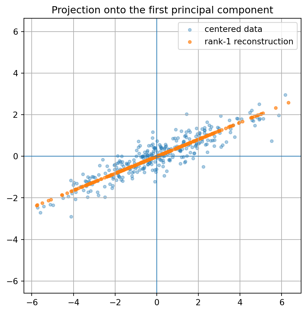
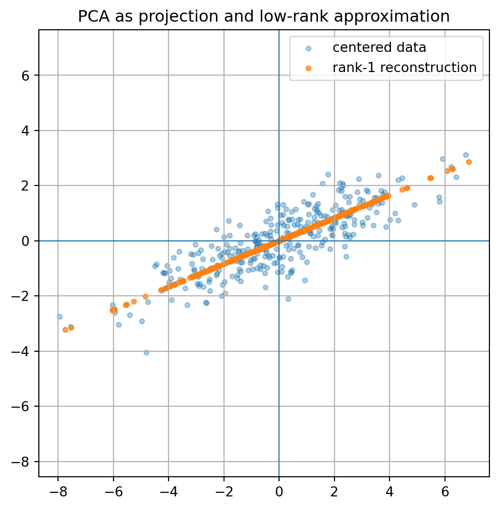
This is projection onto the subspace spanned by the first \(k\) principal components.
For \(k=1\) , each data point is represented by one number.
For larger \(k\) , more structure is preserved.
22.18 Python: PCA projection and reconstruction
= V[:, :1 ]= Xc @ V1= Z @ V1.T= (6 , 6 ))0 ], Xc[:, 1 ], s= 12 , alpha= 0.35 , label= "centered data" )0 ], X_reconstructed[:, 1 ], s= 12 , alpha= 0.65 , label= "rank-1 reconstruction" )0 , linewidth= 0.8 )0 , linewidth= 0.8 )True )"equal" )"Projection onto the first principal component" )
The reconstructed points lie on the best one-dimensional subspace.
22.19 Low-rank structure
Many data matrices are approximately low rank.
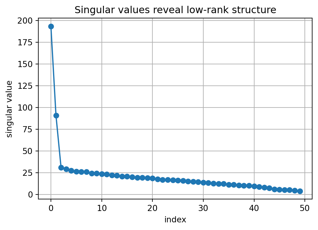
This means that most information can be captured by a small number of singular values and singular vectors.
The truncated SVD
\[
X_k=U_k\Sigma_kV_k^T
\]
is the best rank-\(k\) approximation to \(X\) .
This gives:
compression,
denoising,
latent features,
dimensionality reduction,
recommendation models,
topic models.
22.20 Python: low-rank matrix denoising
= np.random.default_rng(4 )= 80 , 50 = rng.normal(size= m)= rng.normal(size= n)= rng.normal(size= m)= rng.normal(size= n)= 3 * np.outer(u1, v1) + 1.5 * np.outer(u2, v2)= X_true + 2.0 * rng.normal(size= (m, n))= np.linalg.svd(X_noisy, full_matrices= False )def rank_k_approx(U, s, Vt, k):return (U[:, :k] * s[:k]) @ Vt[:k, :]= rank_k_approx(U, s, Vt, 2 )- X_true), np.linalg.norm(X_rank2 - X_true)
(125.66104708574623, 30.439091236936875)
The rank-\(2\) approximation can be closer to the true structure than the noisy matrix.
= (6 , 4 ))= "o" )"index" )"singular value" )True )"Singular values reveal low-rank structure" )
22.21 Images as matrices
A grayscale image is a matrix.
Each entry is a pixel intensity.
A color image can be represented by three matrices: red, green, and blue channels.
Linear algebra operations on images include:
compression,
filtering,
smoothing,
edge detection,
denoising,
dimensionality reduction.
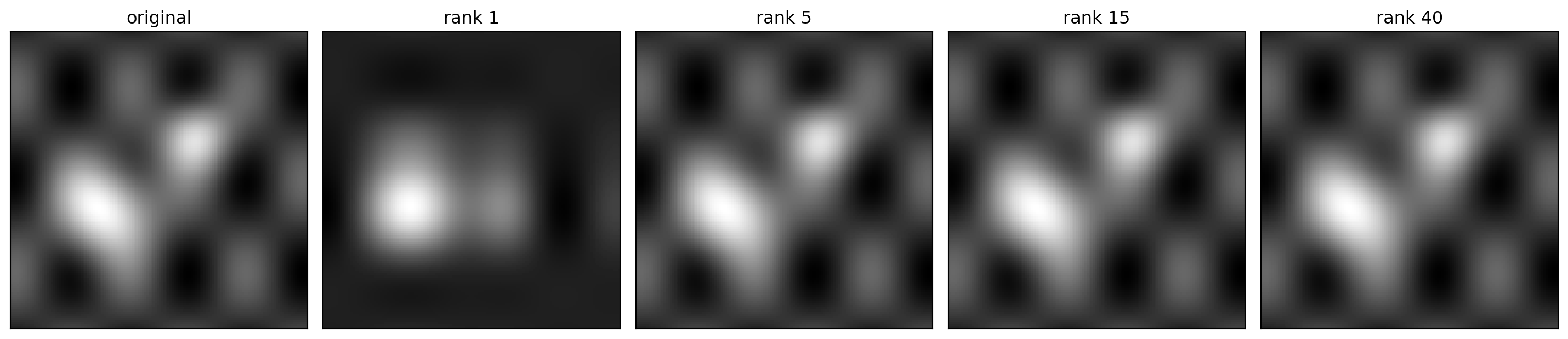
The SVD compresses an image by keeping only the largest singular values.
22.22 Python: synthetic image compression
= 140 = np.linspace(- 1 , 1 , n)= np.linspace(- 1 , 1 , n)= np.meshgrid(x, y)= (- 10 * ((Xgrid+ 0.35 )** 2 + (Ygrid- 0.2 )** 2 ))+ 0.8 * np.exp(- 18 * ((Xgrid- 0.25 )** 2 + (Ygrid+ 0.3 )** 2 ))+ 0.25 * np.sin(8 * Xgrid)* np.cos(5 * Ygrid)= np.linalg.svd(image, full_matrices= False )= [1 , 5 , 15 , 40 ]= plt.subplots(1 , len (ranks)+ 1 , figsize= (15 , 4 ))0 ].imshow(image, cmap= "gray" )0 ].set_title("original" )0 ].set_xticks([])0 ].set_yticks([])for ax, k in zip (axes[1 :], ranks):= rank_k_approx(U, s, Vt, k)= "gray" )f"rank { k} " )
This is a visual example of the SVD as compression.
22.23 Text as vectors
Text can also be represented by vectors.
A simple representation counts word frequencies.
Suppose we have documents and a vocabulary of words.
The document-term matrix is
\[
X_{ij}=
\text{number of times word }j\text{ appears in document }i.
\]
Then:
each row is a document vector,
each column is a word feature,
dot products measure shared word usage,
cosine similarity compares document direction.
More advanced embeddings also represent words, sentences, or documents as vectors, but the geometric ideas are the same: similarity, distance, projection, and dimension.
22.24 A tiny document-term example
Suppose the vocabulary is:
\[
\{\text{linear},\ \text{matrix},\ \text{data},\ \text{model}\}.
\]
A document might be represented as
\[
x=
\begin{bmatrix}
3\\
2\\
0\\
1
\end{bmatrix},
\]
meaning:
3 uses of “linear”,
2 uses of “matrix”,
0 uses of “data”,
1 use of “model”.
Another document is another vector.
Cosine similarity compares their word-use patterns.
22.25 Python: document similarity
= np.array([3 , 2 , 0 , 1 ],2 , 1 , 0 , 0 ],0 , 0 , 3 , 2 ],1 , 1 , 2 , 2 ]= float )= ["linear algebra note" , "matrix exercise" , "data model note" , "mixed document" ]= np.zeros((len (docs), len (docs)))for i in range (len (docs)):for j in range (len (docs)):= cosine_similarity(docs[i], docs[j])
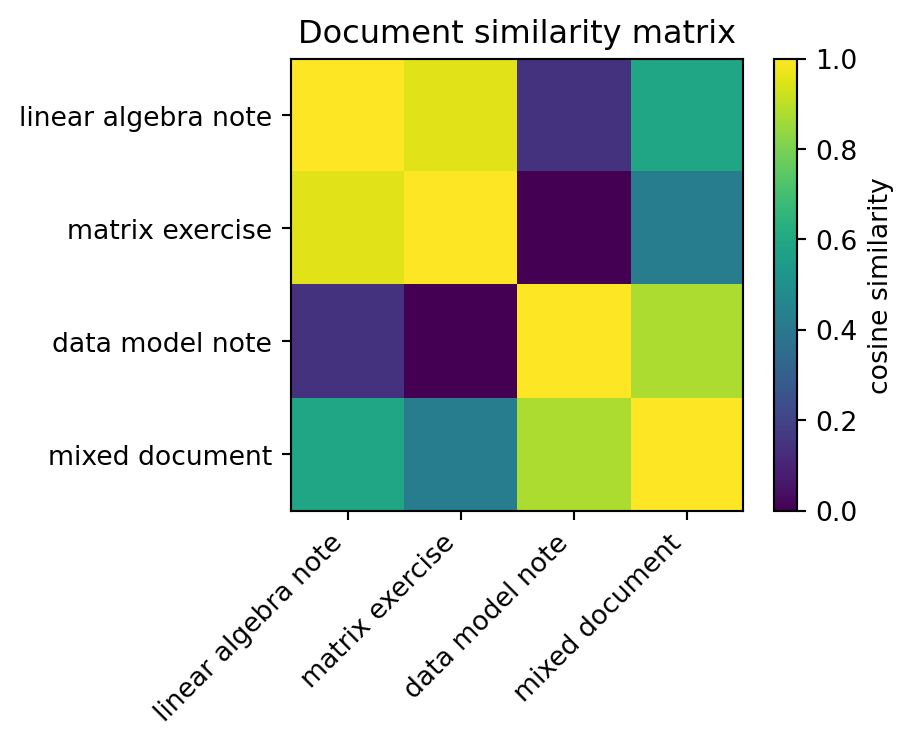
array([[1.        , 0.95618289, 0.14824986, 0.59160798],
       [0.95618289, 1.        , 0.        , 0.42426407],
       [0.14824986, 0.        , 1.        , 0.87705802],
       [0.59160798, 0.42426407, 0.87705802, 1.        ]])
= (5 , 4 ))= "cosine similarity" )range (len (names)), names, rotation= 45 , ha= "right" )range (len (names)), names)"Document similarity matrix" )
The similarity matrix is a Gram matrix of normalized document vectors.
22.26 Recommendation systems as matrix completion
A simple recommendation system can be represented by a user-item matrix.
Rows are users.
Columns are items.
Entries are ratings.
For example,
\[
R_{ij}
\]
might be the rating user \(i\) gives item \(j\) .
Usually many entries are missing.
The goal is to predict missing ratings.
A common idea is that the rating matrix is approximately low rank:
\[
R\approx UV^T.
\]
Here:
rows of \(U\) represent user latent factors,
rows of \(V\) represent item latent factors,
predicted ratings are dot products.
This is another appearance of matrix factorization.
22.27 Low-rank recommendation idea
If user \(i\) has latent vector \(u_i\) and item \(j\) has latent vector \(v_j\) , then the predicted rating is
\[
\hat R_{ij}=u_i\cdot v_j.
\]
So recommendation is built from dot products in a latent feature space.
The model learns hidden coordinates that explain preferences.
This is the same geometric idea as projecting data into a useful lower-dimensional space.
22.28 Graphs as matrices
Graphs can also be represented by matrices.
For a graph with \(n\) nodes, the adjacency matrix is
\[
A_{ij}=
\begin{cases}
1, & \text{if node }i\text{ connects to node }j,\\
0, & \text{otherwise}.
\end{cases}
\]
For an undirected graph, the adjacency matrix is symmetric.
Another important graph matrix is the degree matrix \(D\) , a diagonal matrix whose entries count the number of edges incident to each node.
The graph Laplacian is
\[
L=D-A.
\]
The Laplacian is symmetric positive semidefinite for undirected graphs.
Eigenvectors of graph matrices reveal clusters, connectivity, diffusion, and ranking.
22.29 Python: graph matrix and spectral clustering idea
# A small graph with two clusters = np.array([0 , 1 , 1 , 0 , 0 , 0 ],1 , 0 , 1 , 0 , 0 , 0 ],1 , 1 , 0 , 1 , 0 , 0 ],0 , 0 , 1 , 0 , 1 , 1 ],0 , 0 , 0 , 1 , 0 , 1 ],0 , 0 , 0 , 1 , 1 , 0 ]= float )= A_graph.sum (axis= 1 )= np.diag(degrees)= D_graph - A_graph= np.linalg.eigh(L)
array([-1.30552502e-16,  4.38447187e-01,  3.00000000e+00,  3.00000000e+00,
        3.00000000e+00,  4.56155281e+00])
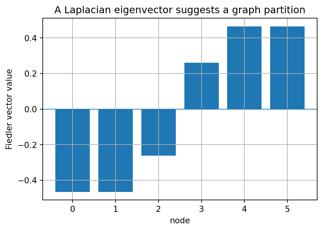
The smallest eigenvalue of the graph Laplacian is \(0\) .
The next eigenvector often reveals a meaningful split in the graph.
= eigvecs[:, 1 ]= (6 , 4 ))len (fiedler)), fiedler)0 , linewidth= 0.8 )"node" )"Fiedler vector value" )"A Laplacian eigenvector suggests a graph partition" )True )
22.30 Neural-network layers as affine maps
A basic neural-network layer has the form
\[
z=Wx+b,
\]
followed by a nonlinear activation
\[
h=\phi(z).
\]
The matrix \(W\) is a linear transformation.
The vector \(b\) is a translation.
The activation \(\phi\) is nonlinear.
Thus a neural-network layer is:
\[
\text{affine map} \quad + \quad \text{nonlinearity}.
\]
Without nonlinearities, a sequence of layers would collapse into one affine map.
For example,
\[
W_2(W_1x+b_1)+b_2
=
(W_2W_1)x+(W_2b_1+b_2).
\]
The nonlinear activation is what allows neural networks to represent more complex functions.
22.31 Python: a small neural-network layer
def relu(z):return np.maximum(0 , z)= np.array([1.0 , - 0.5 ],0.3 , 1.2 ],- 1.0 , 0.7 ]= np.array([0.2 , - 0.1 , 0.5 ])= np.array([2.0 , 1.0 ])= W @ x + b= relu(z)
(array([ 1.7, 1.7, -0.8]), array([1.7, 1.7, 0. ]))
The matrix multiplication creates linear combinations of input features.
The activation changes the geometry by introducing nonlinear behavior.
22.32 Why nonlinearities matter
Suppose a network had only linear layers and no activation functions.
Then
\[
x\mapsto W_1x
\]
followed by
\[
x\mapsto W_2x
\]
followed by
\[
x\mapsto W_3x
\]
would be
\[
x\mapsto W_3W_2W_1x.
\]
This is still just one linear transformation.
Even with biases, a stack of affine transformations is still affine.
Therefore deep learning needs nonlinear activations to go beyond linear algebra.
But the linear parts remain fundamental. They carry most of the parameters and computations.
22.33 Attention as matrix operations
Many modern sequence models use attention-like operations built from matrix products.
A simplified attention computation uses matrices:
\[
Q=XW_Q,
\]
\[
K=XW_K,
\]
\[
V=XW_V.
\]
Then scores are computed by
\[
S=QK^T.
\]
The entry \(S_{ij}\) is a dot product between a query vector and a key vector.
After normalization, the output is a weighted combination of value vectors.
The key linear algebra ideas are:
matrix multiplication,
dot products,
similarity,
normalization,
weighted sums.
This shows again that vector geometry is central to AI.
22.34 Embeddings
An embedding maps an object to a vector.
Objects may be:
words,
sentences,
images,
users,
products,
nodes in a graph,
molecules,
students,
courses.
Once objects are vectors, we can compare them using:
\[
\|x-y\|
\]
or
\[
\frac{x^Ty}{\|x\|\|y\|}.
\]
The goal of embedding is to place similar objects near each other in a meaningful vector space.
Linear algebra gives the geometry of that space.
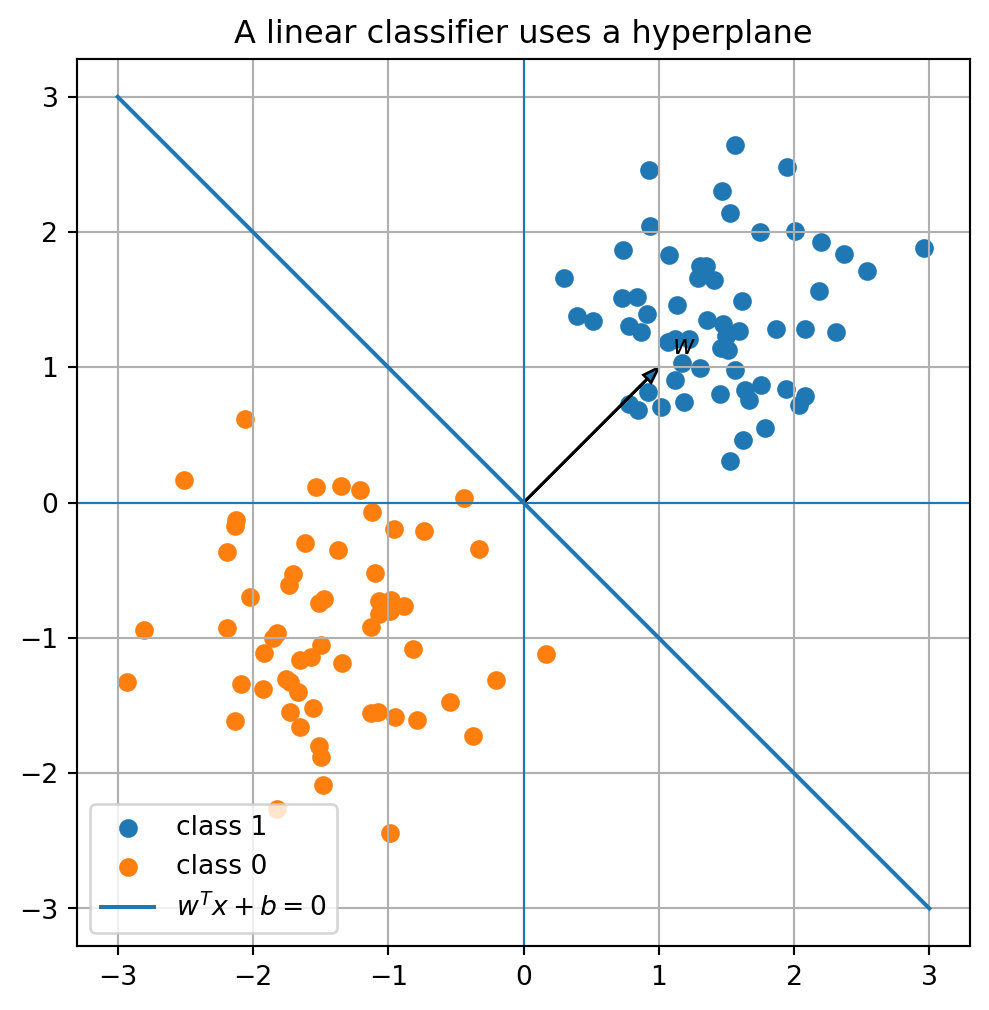
22.35 Classification by linear decision boundaries
A linear classifier separates data using a hyperplane.
For binary classification, a simple rule is
\[
\hat y=
\begin{cases}
1, & w^Tx+b\ge 0,\\
0, & w^Tx+b<0.
\end{cases}
\]
The set
\[
w^Tx+b=0
\]
is a hyperplane.
The vector \(w\) is normal to the hyperplane.
The sign of \(w^Tx+b\) tells which side of the hyperplane the point lies on.
This is another direct use of dot products and geometry.
22.36 Python: linear classifier picture
= np.random.default_rng(5 )= rng.normal(loc= [1.5 , 1.5 ], scale= 0.6 , size= (60 , 2 ))= rng.normal(loc= [- 1.5 , - 1.0 ], scale= 0.6 , size= (60 , 2 ))= np.array([1.0 , 1.0 ])= 0.0 = np.linspace(- 3 , 3 , 100 )= - (w[0 ]* xx + b0) / w[1 ]= (6 , 6 ))0 ], X1[:, 1 ], label= "class 1" )0 ], X2[:, 1 ], label= "class 0" )= "$w^Tx+b=0$" )0 , 0 , w[0 ], w[1 ], head_width= 0.08 , length_includes_head= True )0 ]+ 0.1 , w[1 ]+ 0.1 , "$w$" )0 , linewidth= 0.8 )0 , linewidth= 0.8 )True )"equal" )"A linear classifier uses a hyperplane" )
22.37 Linear algebra ideas that reappear in AI
The same ideas appear repeatedly:
Vector
data point, embedding, feature representation
Matrix
data set, transformation, model layer
Dot product
similarity, prediction, attention score
Norm
length, error, regularization
Projection
approximation, PCA, least squares
Orthogonality
independent directions, stable coordinates
Eigenvectors
principal directions, graph modes, steady states
Singular values
strength of latent components
Low rank
compression, denoising, latent structure
Quadratic form
loss curvature, covariance geometry
Linear algebra is not just a prerequisite for AI.
It is the grammar of many AI computations.
22.38 A small end-to-end example
We now combine several ideas:
Create a data matrix.
Center it.
Use SVD for PCA.
Project to one dimension.
Reconstruct the data.
Measure reconstruction error.
= np.random.default_rng(6 )= rng.multivariate_normal(= [2 , - 1 ],= [[6 , 2.5 ], [2.5 , 1.5 ]],= 300 = X - X.mean(axis= 0 )= np.linalg.svd(Xc, full_matrices= False )= Vt[:1 , :].T= Xc @ V1= Z @ V1.T= np.linalg.norm(Xc - Xc_hat, "fro" )= (6 , 6 ))0 ], Xc[:, 1 ], s= 12 , alpha= 0.35 , label= "centered data" )0 ], Xc_hat[:, 1 ], s= 12 , alpha= 0.7 , label= "rank-1 reconstruction" )0 , linewidth= 0.8 )0 , linewidth= 0.8 )True )"equal" )"PCA as projection and low-rank approximation" )
This one example uses:
data matrices,
centering,
SVD,
projection,
low-rank approximation,
geometric error.
22.39 What this book has built
This book developed a sequence of ideas:
Linear systems describe constraints.
Matrices organize systems and transformations.
Row reduction solves systems.
Matrix algebra describes composition.
Inverses describe reversibility.
Span, basis, and dimension describe linear structure.
Subspaces organize possible solutions and outputs.
Coordinates translate between bases.
Linear transformations move vectors.
Orthogonality gives geometry.
Projection gives best approximation.
QR gives stable orthogonal computation.
Least squares fits data.
Determinants measure volume.
Eigenvectors reveal invariant directions.
Diagonalization explains dynamics.
Symmetric matrices give spectral geometry.
Quadratic forms describe curvature.
SVD reveals low-rank structure.
Together, these ideas form the computational language of linear algebra.
22.40 Algorithmic summary
Given data:
Store observations as rows of a matrix \(X\) .
Center columns by subtracting feature means.
Scale columns if feature units differ strongly.
Use dot products, distances, or cosine similarity to compare rows.
Use matrix factorizations to reveal structure.
Given a data matrix \(X\) :
Center the data:
\[
X_c=X-\mathbf{1}\mu^T.
\]
Compute
\[
X_c=U\Sigma V^T.
\]
Use columns of \(V\) as principal directions.
Project onto the first \(k\) directions:
\[
Z=X_cV_k.
\]
Reconstruct by
\[
\hat X=ZV_k^T.
\]
Given features and responses:
Build a design matrix \(A\) .
Solve
\[
A\beta\approx y
\]
in the least-squares sense. 3. Use QR or SVD for numerical stability. 4. Predict with
\[
\hat y=A\hat\beta.
\]
Given a matrix \(X\) :
Compute
\[
X=U\Sigma V^T.
\]
Keep the first \(k\) singular values and vectors.
Form
\[
X_k=U_k\Sigma_kV_k^T.
\]
Use \(X_k\) for compression, denoising, or latent structure.
22.41 Common mistakes
Mistake 1: treating data matrices as only tables
A data matrix is also a geometric object. Rows are points, columns are features, and matrix operations reveal structure.
Mistake 2: ignoring scaling
Distances and dot products depend on units. Centering and scaling can change the geometry dramatically.
Mistake 3: confusing correlation with causation
Linear algebra can reveal patterns and structure, but interpretation requires context and careful reasoning.
Mistake 4: using high-dimensional distances blindly
In high dimensions, distances can behave unexpectedly. Dimension reduction and normalization often matter.
Mistake 5: keeping too many or too few singular values
Low-rank approximation requires judgment. Too few components lose signal; too many may preserve noise.
Mistake 6: thinking neural networks are only nonlinear magic
Neural networks rely heavily on linear algebra. Matrix multiplication is the main computational engine.
22.42 Chapter summary
Data can be represented as a matrix.
Rows are observations, columns are features.
Dot products measure alignment and support prediction, similarity, and attention.
Norms measure length and error.
Least squares fits linear models by projecting data onto a model space.
PCA uses eigenvectors or the SVD to find directions of maximum variance.
The SVD gives low-rank approximations for compression and denoising.
Images, text, recommendation systems, graphs, and neural-network layers can all be described using vectors and matrices.
Linear algebra provides the grammar of data and AI:
\[
\text{vectors}+\text{matrices}+\text{geometry}+\text{optimization}.
\]
Exercises
A. Data matrices
Suppose
\[
X=
\begin{bmatrix}
1&2&3\\
2&3&5\\
3&4&7\\
4&5&9
\end{bmatrix}.
\]
How many observations are there?
How many features are there?
Compute the column means.
Center the data matrix.
Interpret the rows as points in feature space.
B. Similarity
For
\[
x=
\begin{bmatrix}
1\\2\\3
\end{bmatrix},
\qquad
y=
\begin{bmatrix}
2\\4\\6
\end{bmatrix},
\qquad
z=
\begin{bmatrix}
3\\-2\\1
\end{bmatrix},
\]
Compute \(x\cdot y\) and \(x\cdot z\) .
Compute cosine similarity between \(x\) and \(y\) .
Compute cosine similarity between \(x\) and \(z\) .
Explain the results geometrically.
C. Linear regression
Given data points
\[
(0,1),\ (1,2),\ (2,2),\ (3,4),
\]
Build the design matrix for a line
\[
y=\beta_0+\beta_1t.
\]
Solve the least-squares problem.
Plot the data and fitted line.
Compute residuals.
D. PCA
Generate or use a two-dimensional data set.
Center the data.
Compute the covariance matrix.
Find eigenvalues and eigenvectors.
Compute PCA using the SVD.
Verify that the principal directions agree.
Project data onto the first principal component.
E. Low-rank approximation
Create a matrix \(X\) or use a small image matrix.
Compute its SVD.
Plot singular values.
Construct rank-\(1\) , rank-\(2\) , and rank-\(5\) approximations.
Compute approximation errors.
Explain what information is preserved by larger ranks.
F. Graph matrices
For the adjacency matrix
\[
A=
\begin{bmatrix}
0&1&1&0\\
1&0&1&0\\
1&1&0&1\\
0&0&1&0
\end{bmatrix},
\]
Compute the degree matrix \(D\) .
Compute the graph Laplacian \(L=D-A\) .
Find eigenvalues of \(L\) .
Explain why \(0\) is an eigenvalue.
Interpret the second-smallest eigenvector.
G. Neural-network layers
Let
\[
W=
\begin{bmatrix}
1&-1\\
2&0\\
0&1
\end{bmatrix},
\qquad
b=
\begin{bmatrix}
1\\
0\\
-1
\end{bmatrix}.
\]
For
\[
x=
\begin{bmatrix}
2\\
3
\end{bmatrix},
\]
Compute \(z=Wx+b\) .
Apply ReLU:
\[
h_i=\max(0,z_i).
\]
Explain which part is linear, which part is affine, and which part is nonlinear.
H. Python exercises
Implement cosine similarity.
Center and standardize a data matrix.
Fit a linear regression model using np.linalg.lstsq.
Implement PCA using SVD.
Create a low-rank approximation function.
Compress a synthetic image using SVD.
Build a small graph Laplacian and compute its eigenvectors.
Simulate a neural-network layer.
I. Reflection
Write a short paragraph answering each question.
Why can data be viewed geometrically?
Why are dot products and norms central in AI?
Why does least squares matter for learning from data?
Why does the SVD reveal hidden structure?
What does it mean to say that linear algebra is a language for AI?
Final reflection
Linear algebra is a language of structure.
It begins with equations, but it grows into a way of seeing:
data as points,
matrices as transformations,
subspaces as models,
projections as approximations,
eigenvectors as natural directions,
singular vectors as hidden patterns,
quadratic forms as landscapes,
and algorithms as geometry in motion.
In the age of data and AI, linear algebra is not merely a technical prerequisite. It is a way to translate problems into vectors, matrices, transformations, and optimization. Once a problem is expressed in that language, computation can begin.