3 From Equations to Linear Systems

3.1 Opening question

Suppose several quantities are unknown, but we know some relationships among them.

For example:

traffic flows into and out of intersections,
ingredients must satisfy nutritional requirements,
forces must balance in a mechanical structure,
prices must balance supply and demand,
a data model must match observed measurements.

How do we organize these relationships so that a computer can solve them, and how do we understand the answer geometrically?

This chapter begins the book with the most basic computational problem in linear algebra:

solve several linear equations at the same time.

The key object is a linear system. The key computational idea is elimination. The key geometric idea is intersection.

3.2 Learning goals

After studying this chapter, you should be able to:

Recognize linear and nonlinear equations.
Write a system of linear equations from a verbal or network problem.
Solve small systems by substitution and elimination.
Interpret systems geometrically as intersections of lines, planes, or hyperplanes.
Distinguish among one solution, no solution, and infinitely many solutions.
Write solution sets using parameters.
Check solutions by substitution.
Use Python to solve and visualize simple systems.

3.3 1.1 From numbers to equations

Linear algebra begins with ordinary algebra, but it quickly becomes a language for high-dimensional computation.

We use several number systems:

\[ \mathbb{N} \subset \mathbb{Z} \subset \mathbb{Q} \subset \mathbb{R} \subset \mathbb{C}. \]

In this book, unless otherwise stated, our vectors and matrices have real entries. That means most of our computations take place over \(\mathbb{R}\).

A function of one variable may be linear, such as

\[ f(x)=ax+b, \]

or nonlinear, such as

\[ f(x)=x^2,\qquad f(x)=\sin x,\qquad f(x)=e^x. \]

A function of several variables may also be linear. For example,

\[ f(x_1,x_2)=a_1x_1+a_2x_2+c \]

is linear in the variables \(x_1\) and \(x_2\) except for the constant term. In linear algebra, we usually move the constant to the other side and write equations in the form

\[ a_1x_1+a_2x_2=b. \]

3.4 1.2 Linear equations

Definition: linear equation

A linear equation in variables \(x_1,x_2,\ldots,x_n\) is an equation of the form

\[ a_1x_1+a_2x_2+\cdots+a_nx_n=b, \]

where \(a_1,a_2,\ldots,a_n\) and \(b\) are real numbers.

The numbers \(a_1,a_2,\ldots,a_n\) are called the coefficients.

Examples of linear equations include

\[ 3x+2=0, \]

\[ 2x_1+3x_2=1, \]

and

\[ 2x_1+3x_2-x_3=1. \]

Examples of nonlinear equations include

\[ x^2+y=1, \]

\[ xy=3, \]

and

\[ \sin x+y=0. \]

The reason is that a linear equation only allows variables to appear to the first power and only multiplied by constants. It does not allow products of variables, powers such as \(x^2\), or nonlinear functions such as \(\sin x\).

3.5 1.3 Systems of linear equations

Definition: linear system

A system of linear equations, or linear system, is a collection of linear equations involving the same variables.

For example,

\[ \begin{cases} -2x_1+x_2=2,\\ x_1-2x_2=2 \end{cases} \]

is a system of two linear equations in two variables.

Another example is

\[ \begin{cases} x_1-3x_2-5x_3=1,\\ x_1-x_2-2x_3=0,\\ 3x_1-x_2+x_3=3. \end{cases} \]

A solution of a system is a choice of values for the variables that makes every equation true at the same time.

3.6 1.4 First example: solving by elimination

Consider the system

\[ \begin{cases} x_1-3x_2-5x_3=1,\\ x_1-x_2-2x_3=0,\\ 3x_1-x_2+x_3=3. \end{cases} \]

We solve it by eliminating variables.

Subtract the first equation from the second:

\[ (x_1-x_2-2x_3)-(x_1-3x_2-5x_3)=0-1, \]

\[ 2x_2+3x_3=-1. \]

Subtract three times the first equation from the third:

\[ (3x_1-x_2+x_3)-3(x_1-3x_2-5x_3)=3-3, \]

\[ 8x_2+16x_3=0. \]

Now solve the smaller system

\[ \begin{cases} 2x_2+3x_3=-1,\\ 8x_2+16x_3=0. \end{cases} \]

Divide the second equation by \(8\):

\[ x_2+2x_3=0. \]

\[ x_2=-2x_3. \]

Substitute into \(2x_2+3x_3=-1\):

\[ 2(-2x_3)+3x_3=-1, \]

\[ -x_3=-1, \]

and therefore

\[ x_3=1. \]

Then

\[ x_2=-2. \]

Finally, use the first equation:

\[ x_1-3(-2)-5(1)=1. \]

Thus

\[ x_1+6-5=1, \]

\[ x_1=0. \]

Therefore the solution is

\[ (x_1,x_2,x_3)=(0,-2,1). \]

Always check

Substitute the solution back into the original system:

\[ 0-3(-2)-5(1)=1, \]

\[ 0-(-2)-2(1)=0, \]

\[ 3(0)-(-2)+1=3. \]

All three equations are true.

3.7 1.5 The geometry of a linear system

A linear equation in two variables,

\[ ax+by=c, \]

is a line in the plane.

A solution of a system of two equations is a point that lies on both lines. Therefore, solving a two-variable linear system means finding the intersection of two lines.

There are three possibilities.

3.7.1 One solution

Two nonparallel lines intersect at one point.

Example:

\[ \begin{cases} x+y=3,\\ x-y=1. \end{cases} \]

Adding the equations gives \(2x=4\), so \(x=2\). Then \(y=1\). The solution is

\[ (x,y)=(2,1). \]

3.7.2 No solution

Parallel distinct lines never intersect.

Example:

\[ \begin{cases} x+y=1,\\ x+y=2. \end{cases} \]

No point can satisfy both equations. The system is inconsistent.

3.7.3 Infinitely many solutions

If two equations describe the same line, then every point on that line is a solution.

Example:

\[ \begin{cases} x+y=1,\\ 2x+2y=2. \end{cases} \]

The second equation is just twice the first. The solution set is the whole line

\[ x+y=1. \]

We can write this as

\[ y=1-x. \]

Let \(x=t\). Then

\[ (x,y)=(t,1-t). \]

Here \(t\) is a free parameter.

3.8 1.6 Planes and hyperplanes

A linear equation in three variables,

\[ ax+by+cz=d, \]

is a plane in \(\mathbb{R}^3\).

A system of linear equations in three variables asks for the common intersection of several planes.

Possible solution sets include:

a single point,
a line,
a plane,
no solution.

In general, a linear equation in \(n\) variables,

\[ a_1x_1+a_2x_2+\cdots+a_nx_n=b, \]

is a hyperplane in \(\mathbb{R}^n\).

A linear system asks where several hyperplanes intersect.

The big geometric idea

Solving a linear system means finding an intersection.

In \(\mathbb{R}^2\), we intersect lines.

In \(\mathbb{R}^3\), we intersect planes.

In \(\mathbb{R}^n\), we intersect hyperplanes.

3.9 1.7 Parameters and infinitely many solutions

Consider the system

\[ \begin{cases} x_1-2x_2+3x_3=0,\\ -2x_1+4x_2-6x_3=0. \end{cases} \]

The second equation is \(-2\) times the first, so the two equations contain the same information. We only need

\[ x_1-2x_2+3x_3=0. \]

Solve for the leading variable \(x_1\):

\[ x_1=2x_2-3x_3. \]

The variables \(x_2\) and \(x_3\) are free. Let

\[ x_2=s,\qquad x_3=t. \]

Then

\[ x_1=2s-3t. \]

So the solution set is

\[ \begin{bmatrix} x_1\\ x_2\\ x_3 \end{bmatrix} = \begin{bmatrix} 2s-3t\\ s\\ t \end{bmatrix}. \]

We can rewrite this in vector form:

\[ \begin{bmatrix} x_1\\ x_2\\ x_3 \end{bmatrix} = s \begin{bmatrix} 2\\ 1\\ 0 \end{bmatrix} + t \begin{bmatrix} -3\\ 0\\ 1 \end{bmatrix}. \]

This is the equation of a plane through the origin in \(\mathbb{R}^3\).

3.10 1.8 Inconsistent systems

Now consider

\[ \begin{cases} x_1-2x_2+3x_3=0,\\ -2x_1+4x_2-6x_3=1. \end{cases} \]

The left side of the second equation is \(-2\) times the left side of the first equation. If the first equation is true, then multiplying it by \(-2\) gives

\[ -2x_1+4x_2-6x_3=0. \]

But the second equation says

\[ -2x_1+4x_2-6x_3=1. \]

This is impossible. The system has no solution.

In elimination, this kind of contradiction appears as

\[ 0=1. \]

Whenever a system reduces to a false statement such as \(0=1\), the system is inconsistent.

3.11 1.9 Homogeneous systems

Definition: homogeneous linear system

A linear system is homogeneous if every equation has right-hand side \(0\).

In matrix language, it has the form

\[ Ax=0. \]

A homogeneous system always has at least one solution:

\[ x=0. \]

This is called the trivial solution.

A homogeneous system may have only the trivial solution, or it may have infinitely many solutions.

It can never have no solution, because \(x=0\) always works.

3.12 1.10 Modeling example: traffic flow

Linear systems often come from conservation laws. A basic principle is:

flow in = flow out.

Suppose a small one-way street network has four unknown internal traffic flows:

\[ x_1,\quad x_2,\quad x_3,\quad x_4. \]

Using conservation at each intersection, we obtain one equation per intersection.

From the traffic network in the lecture notes, the equations are

\[ 53+x_1=96+x_4, \]

\[ x_4+121=135+x_3, \]

\[ x_3+45=x_2+78, \]

\[ 152+x_2=62+x_1. \]

Move unknowns to the left and constants to the right:

\[ x_1-x_4=43, \]

\[ -x_3+x_4=14, \]

\[ -x_2+x_3=33, \]

\[ -x_1+x_2=-90. \]

This is a linear system in four unknowns.

Solving gives

\[ x_1=x_4+43,\qquad x_2=x_4-47,\qquad x_3=x_4-14. \]

Let

\[ x_4=t. \]

Then

\[ (x_1,x_2,x_3,x_4)=(t+43,t-47,t-14,t). \]

This system has infinitely many algebraic solutions because one internal flow can be chosen freely.

However, in a real traffic problem we also require all flows to be nonnegative:

\[ x_1\ge 0,\qquad x_2\ge 0,\qquad x_3\ge 0,\qquad x_4\ge 0. \]

These inequalities imply

\[ t\ge 47. \]

Thus the physically meaningful traffic flows are

\[ (x_1,x_2,x_3,x_4)=(t+43,t-47,t-14,t),\qquad t\ge 47. \]

Modeling lesson

Linear algebra often gives a family of possible solutions. The original application may add extra constraints, such as nonnegative traffic, nonnegative mass, probability between \(0\) and \(1\), or integer counts.

3.13 1.11 Row picture and column picture preview

There are two complementary ways to understand a linear system.

Consider

\[ \begin{cases} 3x_1+x_2=7,\\ x_1+2x_2=4. \end{cases} \]

3.13.1 Row picture

Each equation is a line:

\[ 3x_1+x_2=7, \]

\[ x_1+2x_2=4. \]

The solution is the intersection of the two lines.

Solving gives

\[ (x_1,x_2)=(2,1). \]

3.13.2 Column picture

Rewrite the system as

\[ x_1 \begin{bmatrix} 3\\ 1 \end{bmatrix} + x_2 \begin{bmatrix} 1\\ 2 \end{bmatrix} = \begin{bmatrix} 7\\ 4 \end{bmatrix}. \]

The question becomes:

Can we build the vector \(\begin{bmatrix}7\\4\end{bmatrix}\) from the two column vectors \(\begin{bmatrix}3\\1\end{bmatrix}\) and \(\begin{bmatrix}1\\2\end{bmatrix}\)?

The answer is yes:

\[ 2 \begin{bmatrix} 3\\ 1 \end{bmatrix} + 1 \begin{bmatrix} 1\\ 2 \end{bmatrix} = \begin{bmatrix} 7\\ 4 \end{bmatrix}. \]

The row picture emphasizes intersections. The column picture emphasizes linear combinations. Both are essential.

3.14 1.12 A first Python computation

We can use Python to solve small systems numerically.

import numpy as np

A = np.array([
    [1, -3, -5],
    [1, -1, -2],
    [3, -1,  1]
], dtype=float)

b = np.array([1, 0, 3], dtype=float)

x = np.linalg.solve(A, b)
x

array([ 1.48029737e-16, -2.00000000e+00,  1.00000000e+00])

The output should be approximately

\[ \begin{bmatrix} 0\\ -2\\ 1 \end{bmatrix}. \]

We can check the answer by computing \(Ax\):

A @ x

array([1.00000000e+00, 2.22044605e-16, 3.00000000e+00])

This should return the vector \(b\).

3.15 1.13 Visualizing two equations

For a system of two equations in two variables, we can plot the two lines.

Consider

\[ \begin{cases} x+y=3,\\ x-y=1. \end{cases} \]

Solve each equation for \(y\):

\[ y=3-x, \]

\[ y=x-1. \]

import numpy as np
import matplotlib.pyplot as plt

x = np.linspace(-1, 4, 200)

y1 = 3 - x
y2 = x - 1

plt.figure()
plt.plot(x, y1, label="$x+y=3$")
plt.plot(x, y2, label="$x-y=1$")
plt.scatter([2], [1])
plt.text(2.05, 1.05, "(2, 1)")
plt.axhline(0, linewidth=0.8)
plt.axvline(0, linewidth=0.8)
plt.xlabel("$x$")
plt.ylabel("$y$")
plt.legend()
plt.title("Two lines intersecting at one solution")
plt.grid(True)
plt.show()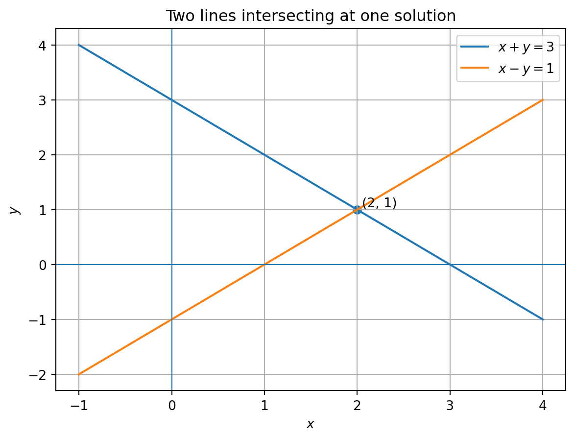

3.16 1.14 Algorithm: elimination by hand

For small systems, the basic elimination strategy is:

Algorithm: elimination

Choose an equation and a variable to eliminate.
Add or subtract multiples of equations to remove that variable from other equations.
Repeat until the system becomes simpler.
Solve the simplified system.
Substitute back to find the remaining variables.
Check the solution in the original system.

In later chapters, we will turn this into the systematic matrix algorithm called Gauss–Jordan elimination.

3.17 1.15 Common mistakes

3.17.1 Mistake 1: forgetting to check all equations

A solution must satisfy every equation, not just one of them.

3.17.2 Mistake 2: confusing no solution with infinitely many solutions

The statement

\[ 0=0 \]

means an equation gave no new information.

The statement

\[ 0=1 \]

means contradiction and no solution.

3.17.3 Mistake 3: treating a free variable as zero

A free variable is not automatically zero. It can be any real number unless the problem gives extra constraints.

3.17.4 Mistake 4: ignoring the application

In traffic, population, mass, or probability problems, a mathematically valid solution may not be physically meaningful unless it satisfies additional constraints.

3.18 1.16 Chapter summary

A linear equation has the form

\[ a_1x_1+\cdots+a_nx_n=b. \]

A linear system is a collection of such equations.

A solution must satisfy all equations at once.

Geometrically:

one equation in two variables is a line,
one equation in three variables is a plane,
one equation in \(n\) variables is a hyperplane,
a system asks for an intersection.

A linear system can have:

exactly one solution,
no solution,
infinitely many solutions.

Homogeneous systems always have at least the zero solution.

Elimination is the first algorithm of linear algebra.

3.19 Exercises

3.19.1 A. Recognizing linear equations

For each equation, determine whether it is linear in the given variables.

\(3x_1-2x_2+7x_3=5\)
\(x_1x_2+x_3=1\)
\(4x-5y=0\)
\(x^2+y=3\)
\(\sin(x)+y=1\)
\(2x_1+3x_2-8=0\)

3.19.2 B. Solving small systems

Solve each system by elimination and check your answer.

\[ \begin{cases} x+y=5,\\ 2x-y=1. \end{cases} \]

\[ \begin{cases} x-2y=3,\\ 2x-4y=6. \end{cases} \]

\[ \begin{cases} x-2y=3,\\ 2x-4y=8. \end{cases} \]

\[ \begin{cases} x_1+x_2+x_3=2,\\ x_1-x_2+2x_3=1,\\ 2x_1+x_2+3x_3=4. \end{cases} \]

3.19.3 C. Geometry

Explain why a system of two equations in two variables can have one solution, no solution, or infinitely many solutions.
Give an example of two equations in two variables whose solution set is the line \(y=2x+1\).
Describe geometrically the solution set of

\[ z=1 \]

as an equation in variables \(x,y,z\).

Describe geometrically what it means for two planes in \(\mathbb{R}^3\) to have infinitely many common points.

3.19.4 D. Parameters

Write the solution set in parametric vector form.

\[ x_1-2x_2+3x_3=0. \]

\[ \begin{cases} x_1+x_2+x_3=1,\\ 2x_1+2x_2+2x_3=2. \end{cases} \]

\[ \begin{cases} x_1+x_2-x_3=0,\\ 2x_1+2x_2-2x_3=1. \end{cases} \]

3.19.5 E. Modeling

A small network has unknown internal flows \(x_1,x_2,x_3\). Conservation of flow gives

\[ x_1+20=x_2+10, \]

\[ x_2+15=x_3+5, \]

\[ x_3= x_1+20. \]

Write the system with all variables on the left and constants on the right.
Solve the system.
Determine whether all flows can be nonnegative.
Interpret your answer.

3.19.6 F. Python

Use np.linalg.solve to solve

\[ \begin{bmatrix} 1 & -3 & -5\\ 1 & -1 & -2\\ 3 & -1 & 1 \end{bmatrix} \begin{bmatrix} x_1\\ x_2\\ x_3 \end{bmatrix} = \begin{bmatrix} 1\\ 0\\ 3 \end{bmatrix}. \]

Check your answer by computing \(Ax-b\).
Plot the two lines

\[ x+y=5,\qquad 2x-y=1. \]

Find their intersection from the plot and from algebra.

3.20 AI-age connection

Linear systems are the first computational language of linear algebra. They appear whenever many constraints must be satisfied simultaneously. In data science and AI, exact systems are often replaced by approximate systems, where there are too many equations and no exact solution. That leads naturally to least squares, regression, projections, QR factorization, and the singular value decomposition. This chapter is the starting point for all of those ideas.