Opening question
Many linear systems in applications do not have exact solutions.
A data set may contain noise. Measurements may be inconsistent. A model may be too simple to fit every observation exactly. In these situations, solving
\[
Ax=b
\]
exactly may be impossible.
But we can still ask for the best approximate solution.
The least-squares problem asks:
Find \(x\) so that \(Ax\) is as close as possible to \(b\) .
That means we want to minimize the error
\[
\|b-Ax\|.
\]
This chapter connects projections, orthogonality, QR factorization, and data fitting. It is one of the most important bridges from linear algebra to statistics, optimization, machine learning, and scientific computing.
Learning goals
After studying this chapter, you should be able to:
Recognize when a linear system is inconsistent.
Formulate the least-squares problem.
Interpret least squares as an orthogonal projection problem.
Derive the normal equations.
Solve least-squares problems using normal equations.
Solve least-squares problems using QR factorization.
Fit lines and polynomials to data.
Interpret residuals and fitted values.
Understand why QR or np.linalg.lstsq is preferred computationally.
Use Python to fit models, plot data, and analyze errors.
15.1 Exact systems versus approximate systems
A linear system
\[
Ax=b
\]
is consistent if \(b\) lies in the column space of \(A\) :
\[
b\in \operatorname{Col}(A).
\]
If \(b\) does not lie in \(\operatorname{Col}(A)\) , then the system has no exact solution.
This is common when \(A\) has more rows than columns. Such systems are called overdetermined systems .
For example, three equations in two unknowns may have no exact solution:
\[
\begin{cases}
x_1+x_2=1,\\
x_1+2x_2=2,\\
x_1+3x_2=2.
\end{cases}
\]
In matrix form,
\[
A=
\begin{bmatrix}
1&1\\
1&2\\
1&3
\end{bmatrix},
\qquad
b=
\begin{bmatrix}
1\\
2\\
2
\end{bmatrix}.
\]
The vector \(b\) may not lie in the plane \(\operatorname{Col}(A)\subseteq \mathbb{R}^3\) .
Instead of solving exactly, we find the vector in \(\operatorname{Col}(A)\) closest to \(b\) .
15.2 The least-squares problem
Given an \(m\times n\) matrix \(A\) and a vector \(b\in\mathbb{R}^m\) , the least-squares problem is to find \(\hat x\in\mathbb{R}^n\) that minimizes
\[
\|b-Ax\|.
\]
Equivalently, it minimizes
\[
\|b-Ax\|^2.
\]
The vector
\[
\hat x
\]
is called a least-squares solution .
The vector
\[
\hat b=A\hat x
\]
is called the fitted vector .
The vector
\[
r=b-A\hat x
\]
is called the residual vector .
The residual measures the error between the observed vector \(b\) and the fitted vector \(\hat b\) .
15.3 Geometry of least squares
The possible vectors \(Ax\) form the column space of \(A\) :
\[
\operatorname{Col}(A)=\{Ax:x\in\mathbb{R}^n\}.
\]
The least-squares problem asks for the point in \(\operatorname{Col}(A)\) closest to \(b\) .
Therefore
\[
A\hat x
\]
must be the orthogonal projection of \(b\) onto \(\operatorname{Col}(A)\) .
Thus the residual
\[
r=b-A\hat x
\]
must be orthogonal to the column space of \(A\) .
Since the columns of \(A\) span \(\operatorname{Col}(A)\) , this means
\[
A^Tr=0.
\]
Substitute \(r=b-A\hat x\) :
\[
A^T(b-A\hat x)=0.
\]
Expanding,
\[
A^Tb-A^TA\hat x=0.
\]
Therefore
\[
A^TA\hat x=A^Tb.
\]
These are the normal equations.
A least-squares solution \(\hat x\) satisfies
\[
A^TA\hat x=A^Tb.
\]
15.4 Why they are called normal equations
The residual
\[
r=b-A\hat x
\]
is orthogonal to the column space of \(A\) .
Another word for orthogonal is normal .
Thus the equation
\[
A^Tr=0
\]
says that the residual is normal to every column of \(A\) .
This is why
\[
A^TA\hat x=A^Tb
\]
is called the system of normal equations.
15.5 A first least-squares example
Consider
\[
A=
\begin{bmatrix}
1&1\\
1&2\\
1&3
\end{bmatrix},
\qquad
b=
\begin{bmatrix}
1\\
2\\
2
\end{bmatrix}.
\]
We solve the normal equations
\[
A^TA\hat x=A^Tb.
\]
Compute
\[
A^TA=
\begin{bmatrix}
1&1&1\\
1&2&3
\end{bmatrix}
\begin{bmatrix}
1&1\\
1&2\\
1&3
\end{bmatrix}
=
\begin{bmatrix}
3&6\\
6&14
\end{bmatrix}.
\]
Also,
\[
A^Tb=
\begin{bmatrix}
1&1&1\\
1&2&3
\end{bmatrix}
\begin{bmatrix}
1\\
2\\
2
\end{bmatrix}
=
\begin{bmatrix}
5\\
11
\end{bmatrix}.
\]
So
\[
\begin{bmatrix}
3&6\\
6&14
\end{bmatrix}
\hat x
=
\begin{bmatrix}
5\\
11
\end{bmatrix}.
\]
Solving gives
\[
\hat x=
\begin{bmatrix}
2/3\\
1/2
\end{bmatrix}.
\]
Thus the fitted model is
\[
\hat y=\frac23+\frac12 x.
\]
15.6 Residual and orthogonality check
For the example above,
\[
\hat x=
\begin{bmatrix}
2/3\\
1/2
\end{bmatrix}.
\]
The fitted vector is
\[
\hat b=A\hat x
=
\begin{bmatrix}
1&1\\
1&2\\
1&3
\end{bmatrix}
\begin{bmatrix}
2/3\\
1/2
\end{bmatrix}
=
\begin{bmatrix}
7/6\\
5/3\\
13/6
\end{bmatrix}.
\]
The residual is
\[
r=b-\hat b
=
\begin{bmatrix}
1\\
2\\
2
\end{bmatrix}
-
\begin{bmatrix}
7/6\\
5/3\\
13/6
\end{bmatrix}
=
\begin{bmatrix}
-1/6\\
1/3\\
-1/6
\end{bmatrix}.
\]
Now check that the residual is orthogonal to the columns of \(A\) :
\[
A^Tr=
\begin{bmatrix}
1&1&1\\
1&2&3
\end{bmatrix}
\begin{bmatrix}
-1/6\\
1/3\\
-1/6
\end{bmatrix}
=
\begin{bmatrix}
0\\
0
\end{bmatrix}.
\]
This confirms the geometric condition.
15.7 Python: solving by normal equations
import numpy as npimport matplotlib.pyplot as plt= np.array([1 , 1 ],1 , 2 ],1 , 3 ]= float )= np.array([1 , 2 , 2 ], dtype= float )= np.linalg.solve(A.T @ A, A.T @ b)= A @ x_hat= b - b_hat@ residual
(array([0.66666667, 0.5       ]),
 array([1.16666667, 1.66666667, 2.16666667]),
 array([-0.16666667,  0.33333333, -0.16666667]),
 array([4.4408921e-16, 8.8817842e-16]))
The final value should be close to zero, confirming that
\[
A^T(b-A\hat x)=0.
\]
15.8 Line fitting
A common least-squares problem is fitting a line to data.
Suppose we have data points
\[
(t_1,y_1),\ldots,(t_m,y_m).
\]
We want to fit a model
\[
y=\beta_0+\beta_1 t.
\]
For each data point,
\[
\beta_0+\beta_1t_i\approx y_i.
\]
This gives the matrix system
\[
\begin{bmatrix}
1&t_1\\
1&t_2\\
\vdots&\vdots\\
1&t_m
\end{bmatrix}
\begin{bmatrix}
\beta_0\\
\beta_1
\end{bmatrix}
\approx
\begin{bmatrix}
y_1\\
y_2\\
\vdots\\
y_m
\end{bmatrix}.
\]
The matrix
\[
A=
\begin{bmatrix}
1&t_1\\
1&t_2\\
\vdots&\vdots\\
1&t_m
\end{bmatrix}
\]
is called the design matrix .
The unknown vector
\[
\beta=
\begin{bmatrix}
\beta_0\\
\beta_1
\end{bmatrix}
\]
contains the model parameters.
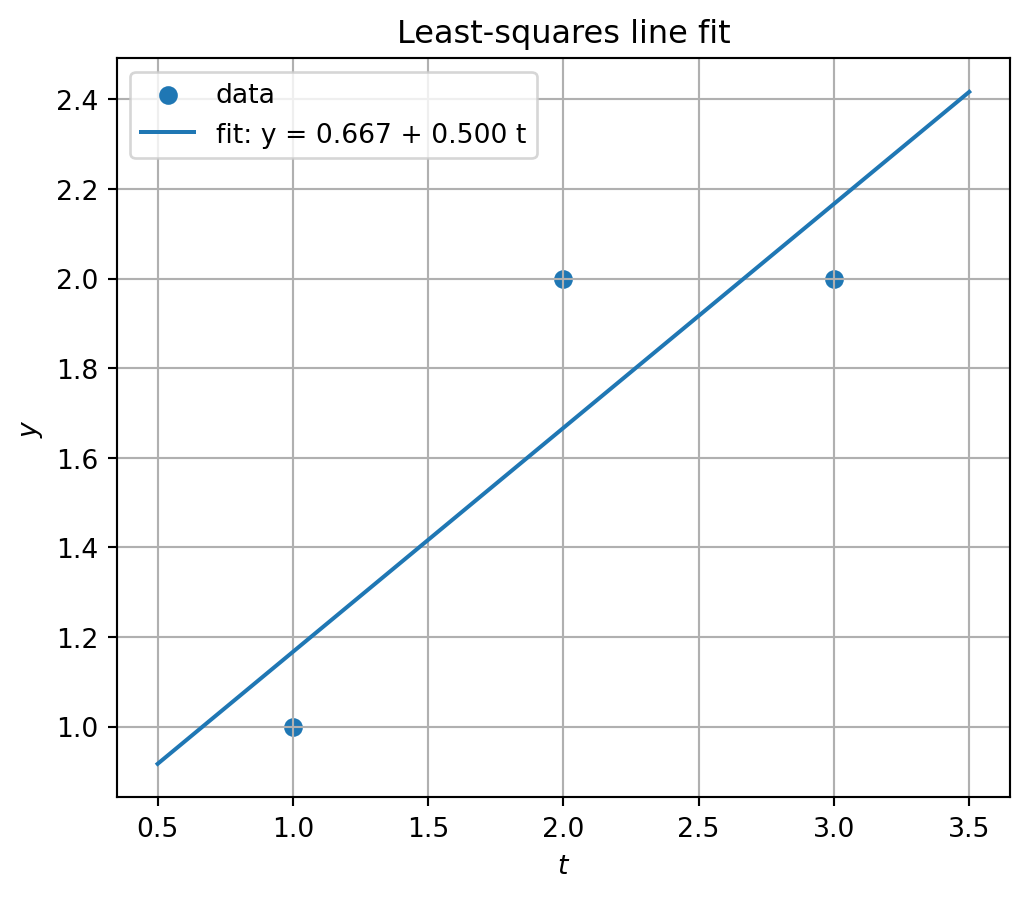
15.9 Python plot: least-squares line
= np.array([1 , 2 , 3 ], dtype= float )= np.array([1 , 2 , 2 ], dtype= float )= np.column_stack([np.ones_like(t), t])= np.linalg.solve(A.T @ A, A.T @ y)= np.linspace(0.5 , 3.5 , 100 )= beta[0 ] + beta[1 ] * t_grid= (6 , 5 ))= "data" )= f"fit: y = { beta[0 ]:.3f} + { beta[1 ]:.3f} t" )"$t$" )"$y$" )True )"Least-squares line fit" )
array([0.66666667, 0.5 ])
The fitted line is
\[
\hat y=\beta_0+\beta_1t.
\]
For this example,
\[
\beta_0=\frac23,
\qquad
\beta_1=\frac12.
\]
15.10 Residuals in data fitting
For each data point, the residual is
\[
r_i=y_i-\hat y_i.
\]
In vector form,
\[
r=y-A\hat\beta.
\]
The sum of squared residuals is
\[
\|r\|^2
=
r_1^2+\cdots+r_m^2.
\]
Least squares chooses the parameters that minimize this quantity.
Root mean squared error
The root mean squared error is
\[
\operatorname{RMSE}
=
\sqrt{\frac{1}{m}\sum_{i=1}^m r_i^2}
=
\frac{\|r\|}{\sqrt{m}}.
\]
This measures the typical size of the residual.
= A @ beta= y - y_hat= np.sum (residuals** 2 )= np.sqrt(np.mean(residuals** 2 ))
(array([-0.16666667,  0.33333333, -0.16666667]),
 0.16666666666666669,
 0.23570226039551584)
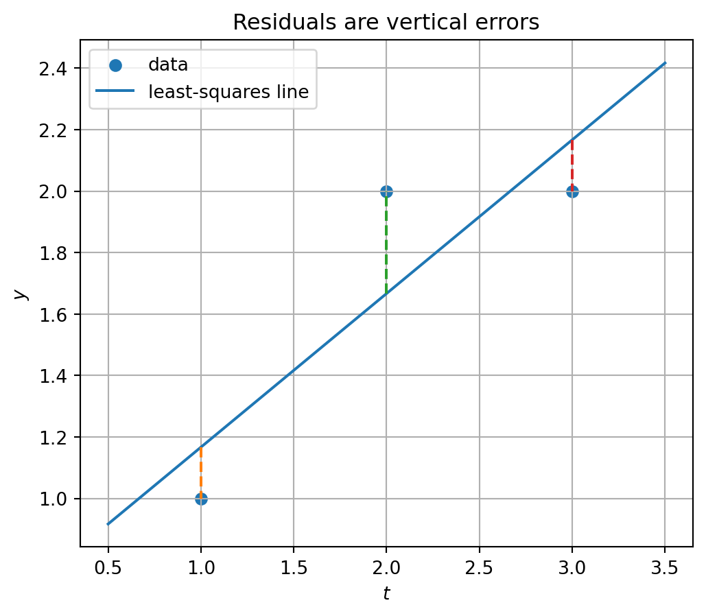
15.11 Visualizing residuals
= (6 , 5 ))= "data" )= "least-squares line" )for ti, yi, yhi in zip (t, y, y_hat):= "--" )"$t$" )"$y$" )True )"Residuals are vertical errors" )
For this line-fitting problem, residuals are vertical distances from data points to the fitted line.
In the vector-space interpretation, the residual vector is orthogonal to the column space of the design matrix.
15.12 QR solution of least squares
The normal equations are mathematically important, but they are not always the best computational method.
If
\[
A=QR,
\]
where \(Q\) has orthonormal columns and \(R\) is upper triangular, then
\[
Ax=QRx.
\]
The least-squares solution satisfies
\[
R\hat x=Q^Tb.
\]
This is easier and usually more stable than solving
\[
A^TA\hat x=A^Tb.
\]
If \(A=QR\) with independent columns, then the least-squares solution is found by solving
\[
R\hat x=Q^Tb.
\]
15.13 Why QR is better than normal equations
The normal equations involve the matrix
\[
A^TA.
\]
This can amplify numerical instability.
In particular, the condition number roughly satisfies
\[
\kappa(A^TA)\approx \kappa(A)^2.
\]
So if \(A\) is ill-conditioned, \(A^TA\) may be much worse.
QR factorization avoids explicitly forming \(A^TA\) and uses orthogonal transformations, which are numerically stable because they preserve lengths.
Use normal equations for theory.
Use QR or np.linalg.lstsq for computation.
15.14 Python: least squares by QR
= np.column_stack([np.ones_like(t), t])= y= np.linalg.qr(A, mode= "reduced" )= np.linalg.solve(R, Q.T @ b)= np.linalg.solve(A.T @ A, A.T @ b)
(array([0.66666667, 0.5 ]), array([0.66666667, 0.5 ]))
The two answers agree for this small example.
15.15 Python: least squares using np.linalg.lstsq
NumPy has a built-in least-squares solver:
= np.linalg.lstsq(A, b, rcond= None )
(array([0.66666667, 0.5       ]),
 array([0.16666667]),
 2,
 array([4.07914333, 0.60049122]))
The function returns:
the least-squares solution,
the residual sum of squares if available,
the rank of the matrix,
the singular values of the matrix.
This is usually the preferred high-level method for least-squares computation in NumPy.
15.16 Polynomial fitting
Least squares is not limited to lines.
Suppose we want to fit a quadratic model
\[
y=\beta_0+\beta_1t+\beta_2t^2.
\]
The design matrix is
\[
A=
\begin{bmatrix}
1&t_1&t_1^2\\
1&t_2&t_2^2\\
\vdots&\vdots&\vdots\\
1&t_m&t_m^2
\end{bmatrix}.
\]
Then we solve
\[
A\beta\approx y
\]
in the least-squares sense.
More generally, a polynomial of degree \(d\) has model
\[
y=\beta_0+\beta_1t+\beta_2t^2+\cdots+\beta_dt^d.
\]
The design matrix has columns
\[
1,\ t,\ t^2,\ \ldots,\ t^d.
\]
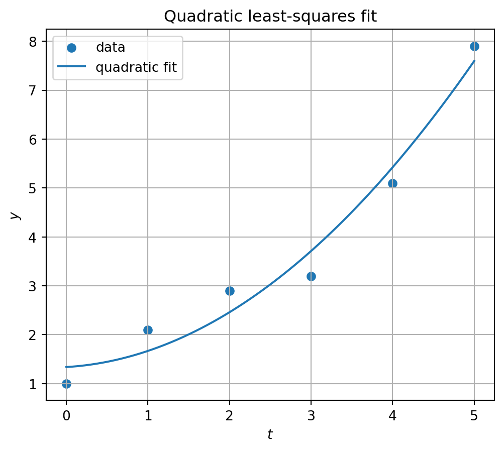
15.17 Python plot: polynomial least squares
= np.array([0 , 1 , 2 , 3 , 4 , 5 ], dtype= float )= np.array([1.0 , 2.1 , 2.9 , 3.2 , 5.1 , 7.9 ], dtype= float )# quadratic design matrix = np.column_stack([np.ones_like(t), t, t** 2 ])= np.linalg.lstsq(A_quad, y, rcond= None )[0 ]= np.linspace(0 , 5 , 200 )= np.column_stack([np.ones_like(t_grid), t_grid, t_grid** 2 ])= A_grid @ beta_quad= (6 , 5 ))= "data" )= "quadratic fit" )"$t$" )"$y$" )True )"Quadratic least-squares fit" )
array([1.33928571, 0.09964286, 0.23035714])
15.18 Overfitting preview
If we use a polynomial with too high a degree, it may fit the training data very closely but behave poorly between or beyond the data points.
This is called overfitting .
From a linear algebra viewpoint, increasing the number of model columns increases the dimension of the model space. A larger model space can reduce training error, but it may also fit noise.
This is one of the central tensions in data science:
simple models may underfit,
overly flexible models may overfit,
useful models balance approximation and generalization.
15.19 Multiple linear regression
Least squares also handles several input variables.
Suppose we model
\[
y=\beta_0+\beta_1x_1+\beta_2x_2+\cdots+\beta_px_p.
\]
For observations
\[
(x_{i1},x_{i2},\ldots,x_{ip},y_i),
\]
the design matrix is
\[
A=
\begin{bmatrix}
1&x_{11}&x_{12}&\cdots&x_{1p}\\
1&x_{21}&x_{22}&\cdots&x_{2p}\\
\vdots&\vdots&\vdots&&\vdots\\
1&x_{m1}&x_{m2}&\cdots&x_{mp}
\end{bmatrix}.
\]
The parameter vector is
\[
\beta=
\begin{bmatrix}
\beta_0\\
\beta_1\\
\vdots\\
\beta_p
\end{bmatrix}.
\]
The least-squares problem is
\[
A\beta\approx y.
\]
This is the matrix form of multiple linear regression.
15.20 Python: multiple regression example
# synthetic data with two predictors = np.array([0 , 1 , 2 , 3 , 4 ], dtype= float )= np.array([1 , 1 , 2 , 2 , 3 ], dtype= float )= np.array([1.1 , 2.0 , 3.2 , 4.0 , 5.1 ], dtype= float )= np.column_stack([np.ones_like(X1), X1, X2])= np.linalg.lstsq(A, y, rcond= None )[0 ]= A @ beta= y - y_hat
(array([0.86666667, 0.86666667, 0.26666667]),
 array([-3.33333333e-02,  1.11022302e-15,  6.66666667e-02,  4.44089210e-16,
        -3.33333333e-02]),
 0.08164965809277304)
The fitted model is
\[
\hat y=\beta_0+\beta_1x_1+\beta_2x_2.
\]
15.21 Rank deficiency and nonunique least-squares solutions
If the columns of \(A\) are linearly independent, then
\[
A^TA
\]
is invertible, and the least-squares solution is unique.
But if the columns of \(A\) are dependent, then \(A^TA\) is not invertible.
In that case, there may be infinitely many least-squares solutions.
Example:
\[
A=
\begin{bmatrix}
1&2\\
2&4\\
3&6
\end{bmatrix}.
\]
The second column is twice the first. The two columns carry the same information.
The model parameters are not uniquely determined.
However, the fitted vector \(A\hat x\) may still be unique as the projection of \(b\) onto \(\operatorname{Col}(A)\) .
15.22 Python: rank-deficient design matrix
= np.array([1 , 2 ],2 , 4 ],3 , 6 ]= float )= np.array([1 , 2 , 2 ], dtype= float )print ("rank:" , np.linalg.matrix_rank(A))= np.linalg.lstsq(A, b, rcond= None )[0 ]
array([0.15714286, 0.31428571])
NumPy returns one least-squares solution, typically the minimum-norm least-squares solution.
The nonuniqueness comes from the nullspace of \(A\) .
15.23 Orthogonal projection and fitted values
Even when the parameter vector is not unique, the fitted vector is determined by the projection:
\[
\hat b=\operatorname{proj}_{\operatorname{Col}(A)}(b).
\]
If \(A\) has independent columns, the projection matrix is
\[
P=A(A^TA)^{-1}A^T.
\]
Then
\[
\hat b=Pb.
\]
The residual is
\[
r=(I-P)b.
\]
The matrices
\[
P
\]
and
\[
I-P
\]
are complementary projection matrices:
\(P\) projects onto \(\operatorname{Col}(A)\) ,\(I-P\) projects onto \(\operatorname{Col}(A)^\perp\) .
15.24 The hat matrix
In statistics, the projection matrix
\[
P=A(A^TA)^{-1}A^T
\]
is often called the hat matrix because it maps observed values to fitted values:
\[
\hat b=Pb.
\]
It puts a “hat” on \(b\) .
For a line-fitting problem,
\[
\hat y=Py.
\]
The diagonal entries of \(P\) are called leverage values. They measure how strongly each observation influences its fitted value.
This is a deeper statistical topic, but the linear algebra idea is simple:
fitted values are projections.
15.25 Python: hat matrix
= np.array([1 , 2 , 3 ], dtype= float )= np.array([1 , 2 , 2 ], dtype= float )= np.column_stack([np.ones_like(t), t])= A @ np.linalg.inv(A.T @ A) @ A.T= P @ y= A @ np.linalg.lstsq(A, y, rcond= None )[0 ]
(array([[ 0.83333333,  0.33333333, -0.16666667],
        [ 0.33333333,  0.33333333,  0.33333333],
        [-0.16666667,  0.33333333,  0.83333333]]),
 array([1.16666667, 1.66666667, 2.16666667]),
 array([1.16666667, 1.66666667, 2.16666667]))
Check projection properties:
@ P, P), np.allclose(P.T, P)
15.26 Weighted least squares preview
Sometimes observations have different reliability.
Weighted least squares minimizes
\[
\sum_{i=1}^m w_i(b_i-(Ax)_i)^2,
\]
where \(w_i>0\) .
In matrix form, this is
\[
\|W^{1/2}(b-Ax)\|^2,
\]
where
\[
W=\operatorname{diag}(w_1,\ldots,w_m).
\]
The normal equations become
\[
A^TWA\hat x=A^TWb.
\]
Weighted least squares is common in statistics, inverse problems, and scientific computing.
15.27 Least squares and optimization
Least squares is also an optimization problem.
Define the objective function
\[
f(x)=\frac12\|Ax-b\|^2.
\]
Expanding,
\[
f(x)=\frac12(Ax-b)^T(Ax-b).
\]
The gradient is
\[
\nabla f(x)=A^T(Ax-b).
\]
At a minimizer \(\hat x\) ,
\[
\nabla f(\hat x)=0.
\]
Thus
\[
A^T(A\hat x-b)=0,
\]
which gives
\[
A^TA\hat x=A^Tb.
\]
So the normal equations also arise from optimization.
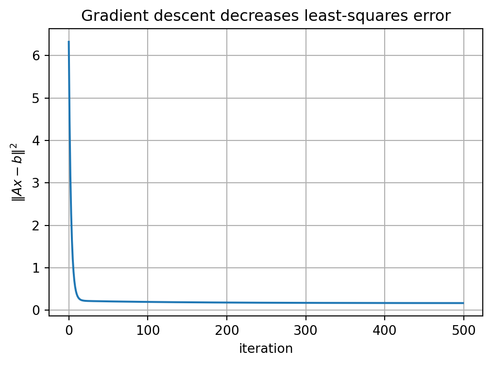
15.28 Gradient descent preview
For large problems, one may solve least-squares problems iteratively.
The gradient descent update for
\[
f(x)=\frac12\|Ax-b\|^2
\]
is
\[
x_{k+1}=x_k-\alpha A^T(Ax_k-b),
\]
where \(\alpha>0\) is a step size.
This is a preview of optimization methods used in machine learning.
= np.array([1 , 1 ],1 , 2 ],1 , 3 ]= float )= np.array([1 , 2 , 2 ], dtype= float )= np.zeros(2 )= 0.01 = []for k in range (500 ):= A.T @ (A @ x - b)= x - alpha * grad@ x - b)** 2 )- 1 ]
(array([0.60518038, 0.52704792]), 0.16829370273548136)
= (6 , 4 ))"iteration" )"$ \\ |Ax-b \\ |^2$" )True )"Gradient descent decreases least-squares error" )
15.29 Algorithmic summary
Given \(A\) and \(b\) :
Form \(A^TA\) and \(A^Tb\) .
Solve
\[
A^TA\hat x=A^Tb.
\]
Compute the fitted vector
\[
\hat b=A\hat x.
\]
Compute the residual
\[
r=b-\hat b.
\]
Given \(A\) with independent columns:
Compute
\[
A=QR.
\]
Solve
\[
R\hat x=Q^Tb.
\]
Compute
\[
\hat b=A\hat x.
\]
Given data \((t_i,y_i)\) :
Build the design matrix
\[
A=
\begin{bmatrix}
1&t_1\\
1&t_2\\
\vdots&\vdots\\
1&t_m
\end{bmatrix}.
\]
Solve
\[
A\beta\approx y
\]
in the least-squares sense. 3. The fitted line is
\[
\hat y=\beta_0+\beta_1t.
\]
15.30 Common mistakes
Mistake 1: expecting an exact solution
Least squares is used when \(Ax=b\) may not be exactly solvable.
The goal is to minimize error, not eliminate it.
Mistake 2: forgetting the residual orthogonality condition
At the least-squares solution,
\[
A^T(b-A\hat x)=0.
\]
The residual is orthogonal to the column space of \(A\) .
Mistake 3: solving \(A\hat x=b\) when the system is inconsistent
For overdetermined data-fitting problems, solve the least-squares problem instead.
Mistake 4: using normal equations blindly
Normal equations are important theoretically, but QR or np.linalg.lstsq is usually preferred computationally.
Mistake 5: confusing residuals with fitted values
The fitted vector is
\[
\hat b=A\hat x.
\]
The residual vector is
\[
r=b-\hat b.
\]
Mistake 6: ignoring rank deficiency
If the columns of \(A\) are dependent, the least-squares solution may not be unique.
15.31 Chapter summary
The least-squares problem is to minimize
\[
\|b-Ax\|.
\]
Geometrically, \(A\hat x\) is the projection of \(b\) onto \(\operatorname{Col}(A)\) .
The residual
\[
r=b-A\hat x
\]
is orthogonal to the column space:
\[
A^Tr=0.
\]
This leads to the normal equations:
\[
A^TA\hat x=A^Tb.
\]
If \(A\) has independent columns, the least-squares solution is unique.
Using QR factorization,
\[
A=QR,
\]
the least-squares solution can be found by solving
\[
R\hat x=Q^Tb.
\]
In data fitting, the design matrix encodes the model, the coefficient vector contains parameters, and the fitted vector is a projection.
Least squares is the foundation of regression, approximation, optimization, and many machine learning algorithms.
Exercises
A. Normal equations
For each \(A\) and \(b\) , form the normal equations and solve for \(\hat x\) .
\[
A=
\begin{bmatrix}
1&1\\
1&2\\
1&3
\end{bmatrix},
\qquad
b=
\begin{bmatrix}
1\\
2\\
2
\end{bmatrix}.
\]
\[
A=
\begin{bmatrix}
1\\
2\\
2
\end{bmatrix},
\qquad
b=
\begin{bmatrix}
2\\
1\\
3
\end{bmatrix}.
\]
\[
A=
\begin{bmatrix}
1&0\\
0&1\\
1&1
\end{bmatrix},
\qquad
b=
\begin{bmatrix}
2\\
1\\
4
\end{bmatrix}.
\]
B. Residuals
For each problem in Exercise A:
Compute \(\hat b=A\hat x\) .
Compute \(r=b-\hat b\) .
Verify that \(A^Tr=0\) .
Compute \(\|r\|\) .
C. Line fitting
Fit a line
\[
y=\beta_0+\beta_1t
\]
to each data set.
\[
(1,1),\ (2,2),\ (3,2)
\]
\[
(0,1),\ (1,2),\ (2,2),\ (3,4)
\]
\[
(-1,0),\ (0,1),\ (1,1),\ (2,3)
\]
For each, compute the fitted values and residuals.
D. Polynomial fitting
Fit a quadratic model
\[
y=\beta_0+\beta_1t+\beta_2t^2
\]
to the data
\[
(0,1),\ (1,2.1),\ (2,2.9),\ (3,3.2),\ (4,5.1),\ (5,7.9).
\]
Build the design matrix.
Compute the least-squares coefficients.
Plot the fitted curve.
Compute the residual norm.
E. QR least squares
For
\[
A=
\begin{bmatrix}
1&1\\
1&2\\
1&3
\end{bmatrix},
\qquad
b=
\begin{bmatrix}
1\\
2\\
2
\end{bmatrix},
\]
Compute a QR factorization of \(A\) .
Solve
\[
R\hat x=Q^Tb.
\]
Compare with the normal-equation solution.
Verify that the residual is orthogonal to \(\operatorname{Col}(A)\) .
F. Rank deficiency
Let
\[
A=
\begin{bmatrix}
1&2\\
2&4\\
3&6
\end{bmatrix}.
\]
Explain why the columns are dependent.
Determine the rank of \(A\) .
Explain why \(A^TA\) is not invertible.
Use Python to compute a least-squares solution for a vector \(b\) of your choice.
Explain why the parameter vector may not be unique.
G. Python exercises
Write a Python function that solves least squares using normal equations.
Write a Python function that solves least squares using QR.
Compare both functions with np.linalg.lstsq.
Fit a line to a noisy data set.
Fit a quadratic curve to a noisy data set.
Plot residuals for a fitted model.
Implement gradient descent for least squares and plot the error over iterations.
H. Reflection
Write a short paragraph answering each question.
Why is least squares a projection problem?
Why is the residual orthogonal to the column space?
Why are normal equations important theoretically?
Why is QR usually better computationally?
How does least squares connect linear algebra to statistics and AI?
AI-age connection
Least squares is one of the most important mathematical ideas in data science and artificial intelligence. Linear regression, polynomial regression, signal approximation, model calibration, inverse problems, and optimization all begin with the question of best approximation. In high-dimensional AI systems, least-squares geometry appears inside training algorithms, embeddings, projections, and error minimization. The core idea is simple but powerful: find the closest point in a model space.