Opening question
In the previous chapters, orthogonality made geometry simpler.
Projection onto a line was easy when the direction vector was known. Projection onto a subspace was especially simple when the basis was orthonormal:
\[
\operatorname{proj}_W(b)=\sum_{j=1}^k (b\cdot q_j)q_j.
\]
So a natural question appears:
Given a set of independent vectors, can we replace them with an orthonormal set that spans the same subspace?
The answer is yes.
The method is called the Gram–Schmidt process .
The matrix version of this process is the QR factorization :
\[
A=QR.
\]
Here \(Q\) has orthonormal columns, and \(R\) is upper triangular.
QR factorization is one of the central tools of computational linear algebra. It is used in least squares, numerical stability, eigenvalue algorithms, data fitting, orthogonalization, and many modern matrix algorithms.
Learning goals
After studying this chapter, you should be able to:
Explain why orthonormal bases simplify projection.
Apply the Gram–Schmidt process to a set of independent vectors.
Construct an orthogonal basis from a given basis.
Normalize an orthogonal basis to obtain an orthonormal basis.
Understand the matrix factorization \(A=QR\) .
Compute a QR factorization by Gram–Schmidt.
Use QR factorization to compute projections.
Use QR factorization to solve least-squares problems.
Understand why numerical orthogonality matters.
Use Python to compute and check QR factorizations.
14.1 Why orthonormal bases are valuable
Suppose
\[
W=\operatorname{span}\{q_1,\ldots,q_k\},
\]
where \(q_1,\ldots,q_k\) are orthonormal.
Then projection is easy:
\[
\operatorname{proj}_W(b)
=
(q_1\cdot b)q_1+\cdots+(q_k\cdot b)q_k.
\]
Coordinates are also easy. If
\[
w=c_1q_1+\cdots+c_kq_k,
\]
then
\[
c_j=w\cdot q_j.
\]
This works because
\[
q_i\cdot q_j=0
\]
when \(i\ne j\) , and
\[
q_j\cdot q_j=1.
\]
Thus orthonormal bases turn many linear algebra problems into dot products.
14.2 The problem
Suppose we start with independent vectors
\[
a_1,a_2,\ldots,a_k.
\]
They may not be orthogonal.
We want to construct vectors
\[
q_1,q_2,\ldots,q_k
\]
such that:
\(q_1,\ldots,q_k\) are orthonormal,for every \(j\) ,
\[
\operatorname{span}\{q_1,\ldots,q_j\}
=
\operatorname{span}\{a_1,\ldots,a_j\}.
\]
This means we keep the same growing sequence of subspaces, but we replace the original vectors with orthonormal directions.
The Gram–Schmidt process does this one vector at a time.
14.3 The first step
Start with a nonzero vector \(a_1\) .
Set
\[
u_1=a_1.
\]
Then normalize:
\[
q_1=\frac{u_1}{\|u_1\|}.
\]
Now \(q_1\) is a unit vector in the same direction as \(a_1\) .
14.4 The second step
Now consider \(a_2\) .
We want to remove the part of \(a_2\) that lies in the direction of \(q_1\) .
The projection of \(a_2\) onto \(\operatorname{span}\{q_1\}\) is
\[
(a_2\cdot q_1)q_1.
\]
Define
\[
u_2=a_2-(a_2\cdot q_1)q_1.
\]
Then \(u_2\) is orthogonal to \(q_1\) .
To see this, compute
\[
u_2\cdot q_1
=
\left(a_2-(a_2\cdot q_1)q_1\right)\cdot q_1.
\]
Using linearity of the dot product,
\[
u_2\cdot q_1
=
a_2\cdot q_1-(a_2\cdot q_1)(q_1\cdot q_1).
\]
Since \(q_1\) is a unit vector,
\[
q_1\cdot q_1=1.
\]
Therefore
\[
u_2\cdot q_1
=
a_2\cdot q_1-(a_2\cdot q_1)=0.
\]
Now normalize:
\[
q_2=\frac{u_2}{\|u_2\|}.
\]
14.5 The general Gram–Schmidt process
At step \(j\) , subtract from \(a_j\) its projections onto the previously constructed orthonormal vectors.
Define
\[
u_j
=
a_j
-
(a_j\cdot q_1)q_1
-
(a_j\cdot q_2)q_2
-
\cdots
-
(a_j\cdot q_{j-1})q_{j-1}.
\]
Then normalize:
\[
q_j=\frac{u_j}{\|u_j\|}.
\]
Given independent vectors \(a_1,\ldots,a_k\) , define
\[
u_1=a_1,\qquad q_1=\frac{u_1}{\|u_1\|}.
\]
For \(j=2,\ldots,k\) , define
\[
u_j
=
a_j-\sum_{i=1}^{j-1}(a_j\cdot q_i)q_i,
\]
and
\[
q_j=\frac{u_j}{\|u_j\|}.
\]
Then \(q_1,\ldots,q_k\) are orthonormal and span the same subspace as \(a_1,\ldots,a_k\) .
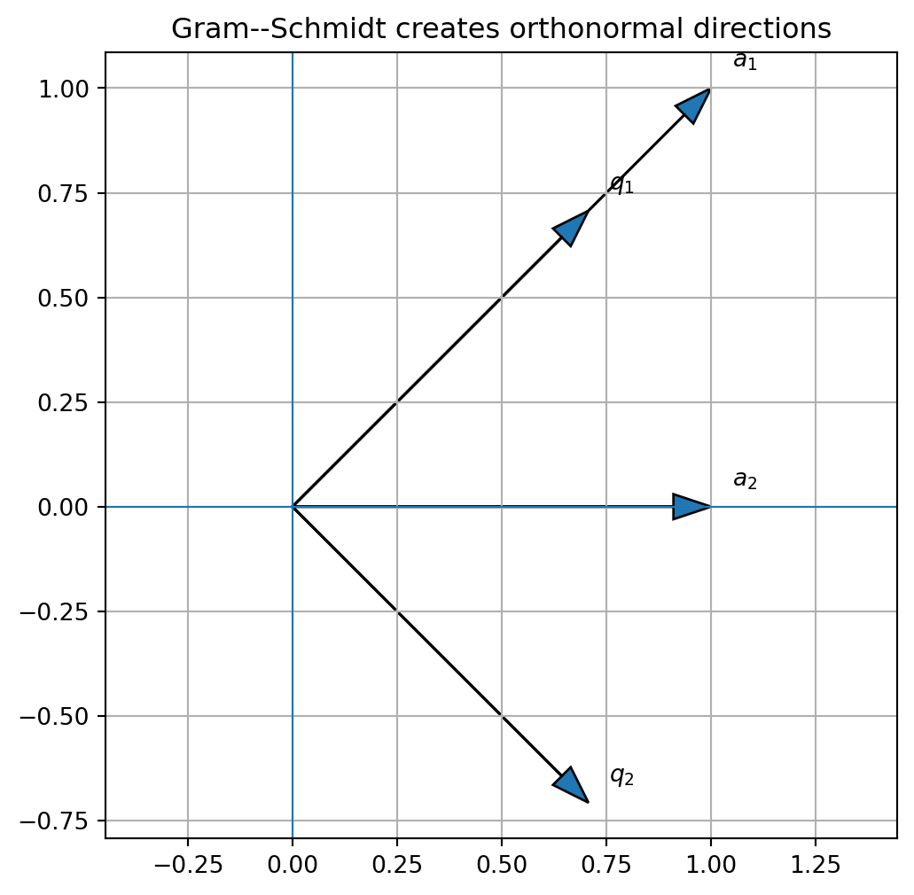
14.6 Example in \(\mathbb{R}^2\)
Let
\[
a_1=
\begin{bmatrix}
1\\
1
\end{bmatrix},
\qquad
a_2=
\begin{bmatrix}
1\\
0
\end{bmatrix}.
\]
First,
\[
u_1=a_1=
\begin{bmatrix}
1\\
1
\end{bmatrix}.
\]
The norm is
\[
\|u_1\|=\sqrt{2}.
\]
So
\[
q_1=
\frac{1}{\sqrt{2}}
\begin{bmatrix}
1\\
1
\end{bmatrix}.
\]
Now compute
\[
u_2=a_2-(a_2\cdot q_1)q_1.
\]
Since
\[
a_2\cdot q_1=
\begin{bmatrix}
1\\
0
\end{bmatrix}
\cdot
\frac{1}{\sqrt{2}}
\begin{bmatrix}
1\\
1
\end{bmatrix}
=
\frac{1}{\sqrt{2}},
\]
we get
\[
(a_2\cdot q_1)q_1
=
\frac{1}{\sqrt{2}}
\frac{1}{\sqrt{2}}
\begin{bmatrix}
1\\
1
\end{bmatrix}
=
\frac12
\begin{bmatrix}
1\\
1
\end{bmatrix}.
\]
Therefore
\[
u_2=
\begin{bmatrix}
1\\
0
\end{bmatrix}
-
\frac12
\begin{bmatrix}
1\\
1
\end{bmatrix}
=
\begin{bmatrix}
1/2\\
-1/2
\end{bmatrix}.
\]
Normalize:
\[
\|u_2\|=\sqrt{\frac14+\frac14}=\frac{1}{\sqrt{2}}.
\]
Thus
\[
q_2=
\frac{u_2}{\|u_2\|}
=
\frac{1}{\sqrt{2}}
\begin{bmatrix}
1\\
-1
\end{bmatrix}.
\]
So an orthonormal basis is
\[
q_1=
\frac{1}{\sqrt{2}}
\begin{bmatrix}
1\\
1
\end{bmatrix},
\qquad
q_2=
\frac{1}{\sqrt{2}}
\begin{bmatrix}
1\\
-1
\end{bmatrix}.
\]
14.7 Python plot: Gram–Schmidt in \(\mathbb{R}^2\)
import numpy as npimport matplotlib.pyplot as plt= np.array([1 , 1 ], dtype= float )= np.array([1 , 0 ], dtype= float )= a1 / np.linalg.norm(a1)= a2 - np.dot(a2, q1) * q1= u2 / np.linalg.norm(u2)= (6 , 6 ))for v, label in [(a1, "$a_1$" ), (a2, "$a_2$" ), (q1, "$q_1$" ), (q2, "$q_2$" )]:0 , 0 , v[0 ], v[1 ], head_width= 0.06 , length_includes_head= True )0 ] + 0.05 , v[1 ] + 0.05 , label)0 , linewidth= 0.8 )0 , linewidth= 0.8 )True )"equal" )"Gram--Schmidt creates orthonormal directions" )print ("q1 dot q2 =" , np.dot(q1, q2))print ("norm q1 =" , np.linalg.norm(q1))print ("norm q2 =" , np.linalg.norm(q2))
q1 dot q2 = 2.7817808468846267e-16
norm q1 = 0.9999999999999999
norm q2 = 1.0
14.8 Example in \(\mathbb{R}^3\)
Let
\[
a_1=
\begin{bmatrix}
1\\
1\\
0
\end{bmatrix},
\qquad
a_2=
\begin{bmatrix}
1\\
0\\
1
\end{bmatrix},
\qquad
a_3=
\begin{bmatrix}
0\\
1\\
1
\end{bmatrix}.
\]
Gram–Schmidt produces an orthonormal basis for \(\mathbb{R}^3\) .
The first vector is
\[
q_1=
\frac{1}{\sqrt{2}}
\begin{bmatrix}
1\\
1\\
0
\end{bmatrix}.
\]
Then
\[
u_2=a_2-(a_2\cdot q_1)q_1.
\]
After computing \(u_2\) , normalize it to get \(q_2\) .
Then
\[
u_3=a_3-(a_3\cdot q_1)q_1-(a_3\cdot q_2)q_2.
\]
Normalize \(u_3\) to get \(q_3\) .
The algebra can become long by hand, but the process is systematic.
14.9 Python implementation of Gram–Schmidt
def gram_schmidt(A, tol= 1e-12 ):""" Classical Gram--Schmidt for the columns of A. Returns Q and R such that A = Q R when columns are independent. """ = np.array(A, dtype= float )= A.shape= np.zeros((m, n))= np.zeros((n, n))for j in range (n):= A[:, j].copy()for i in range (j):= np.dot(Q[:, i], A[:, j])= v - R[i, j] * Q[:, i]= np.linalg.norm(v)if R[j, j] < tol:raise ValueError ("Columns are linearly dependent or nearly dependent." )= v / R[j, j]return Q, R= np.array([1 , 1 , 0 ],1 , 0 , 1 ],0 , 1 , 1 ]= float )= gram_schmidt(A)
(array([[ 0.70710678,  0.40824829, -0.57735027],
        [ 0.70710678, -0.40824829,  0.57735027],
        [ 0.        ,  0.81649658,  0.57735027]]),
 array([[1.41421356, 0.70710678, 0.70710678],
        [0.        , 1.22474487, 0.40824829],
        [0.        , 0.        , 1.15470054]]))
Check orthonormality:
array([[ 1.00000000e+00,  1.03018891e-16,  1.51811967e-16],
       [ 1.03018891e-16,  1.00000000e+00, -1.59104334e-16],
       [ 1.51811967e-16, -1.59104334e-16,  1.00000000e+00]])
Check reconstruction:
array([[1.00000000e+00, 1.00000000e+00, 4.02426802e-17],
       [1.00000000e+00, 1.73428748e-19, 1.00000000e+00],
       [0.00000000e+00, 1.00000000e+00, 1.00000000e+00]])
The matrix \(Q^TQ\) should be close to the identity matrix, and \(QR\) should reproduce \(A\) .
14.10 From Gram–Schmidt to QR factorization
Suppose
\[
A=
\begin{bmatrix}
|&|&&|\\
a_1&a_2&\cdots&a_n\\
|&|&&|
\end{bmatrix}
\]
has linearly independent columns.
Gram–Schmidt constructs orthonormal vectors
\[
q_1,\ldots,q_n.
\]
Let
\[
Q=
\begin{bmatrix}
|&|&&|\\
q_1&q_2&\cdots&q_n\\
|&|&&|
\end{bmatrix}.
\]
Each original column \(a_j\) can be written as a linear combination of \(q_1,\ldots,q_j\) :
\[
a_j=r_{1j}q_1+r_{2j}q_2+\cdots+r_{jj}q_j.
\]
Because only \(q_1,\ldots,q_j\) appear, the coefficient matrix is upper triangular:
\[
R=
\begin{bmatrix}
r_{11}&r_{12}&\cdots&r_{1n}\\
0&r_{22}&\cdots&r_{2n}\\
\vdots&\vdots&\ddots&\vdots\\
0&0&\cdots&r_{nn}
\end{bmatrix}.
\]
Thus
\[
A=QR.
\]
If \(A\) has linearly independent columns, then
\[
A=QR,
\]
where \(Q\) has orthonormal columns and \(R\) is upper triangular.
14.11 How to read \(A=QR\)
The factorization
\[
A=QR
\]
means that the columns of \(A\) are built from the orthonormal columns of \(Q\) .
Since \(Q\) has orthonormal columns,
\[
Q^TQ=I.
\]
Since \(R\) is upper triangular, it stores the coordinates needed to express each \(a_j\) using the orthonormal basis vectors created so far.
The diagonal entries of \(R\) are the lengths of the new orthogonal components:
\[
r_{jj}=\|u_j\|.
\]
The off-diagonal entries are dot products:
\[
r_{ij}=q_i^Ta_j
\qquad i<j.
\]
14.12 Reduced and full QR factorization
If \(A\) is an \(m\times n\) matrix with independent columns and \(m\ge n\) , then the reduced QR factorization is
\[
A=QR,
\]
where
\[
Q
\]
is \(m\times n\) with orthonormal columns, and
\[
R
\]
is \(n\times n\) upper triangular.
A full QR factorization extends \(Q\) to an \(m\times m\) orthogonal matrix:
\[
A=Q_{\text{full}}R_{\text{full}}.
\]
For most least-squares and data applications, the reduced QR factorization is the most useful version.
14.13 QR and projection
If the columns of \(Q\) are orthonormal, then the projection onto \(\operatorname{Col}(Q)\) is
\[
P=QQ^T.
\]
Since
\[
A=QR
\]
and \(R\) is invertible when the columns of \(A\) are independent,
\[
\operatorname{Col}(A)=\operatorname{Col}(Q).
\]
Therefore the projection onto \(\operatorname{Col}(A)\) is also
\[
P=QQ^T.
\]
This avoids the more complicated formula
\[
P=A(A^TA)^{-1}A^T.
\]
If \(A=QR\) with \(Q\) having orthonormal columns, then
\[
\operatorname{proj}_{\operatorname{Col}(A)}(b)=QQ^Tb.
\]
14.14 QR and least squares
The least-squares problem asks for \(\hat x\) minimizing
\[
\|b-Ax\|.
\]
If
\[
A=QR,
\]
then
\[
Ax=QRx.
\]
Because \(Q\) has orthonormal columns, the least-squares solution satisfies
\[
R\hat x=Q^Tb.
\]
Thus we solve the triangular system
\[
R\hat x=Q^Tb.
\]
If \(A=QR\) has independent columns, then the least-squares solution of \(Ax\approx b\) is found by solving
\[
R\hat x=Q^Tb.
\]
This is often more stable than solving the normal equations
\[
A^TA\hat x=A^Tb.
\]
14.15 Example: least squares by QR
Let
\[
A=
\begin{bmatrix}
1&1\\
1&2\\
1&3
\end{bmatrix},
\qquad
b=
\begin{bmatrix}
1\\
2\\
2
\end{bmatrix}.
\]
The columns of \(A\) are independent.
Compute
\[
A=QR.
\]
Then solve
\[
R\hat x=Q^Tb.
\]
The fitted vector is
\[
\hat b=A\hat x.
\]
The error
\[
e=b-\hat b
\]
is orthogonal to \(\operatorname{Col}(A)\) .
14.16 Python: least squares by QR
= np.array([1 , 1 ],1 , 2 ],1 , 3 ]= float )= np.array([1 , 2 , 2 ], dtype= float )= np.linalg.qr(A, mode= "reduced" )= np.linalg.solve(R, Q.T @ b)= A @ x_hat= b - b_hat@ error
(array([0.66666667, 0.5       ]),
 array([1.16666667, 1.66666667, 2.16666667]),
 array([-0.16666667,  0.33333333, -0.16666667]),
 array([ 0.0000000e+00, -4.4408921e-16]))
The final output should be close to zero, showing that the error is orthogonal to the columns of \(A\) .
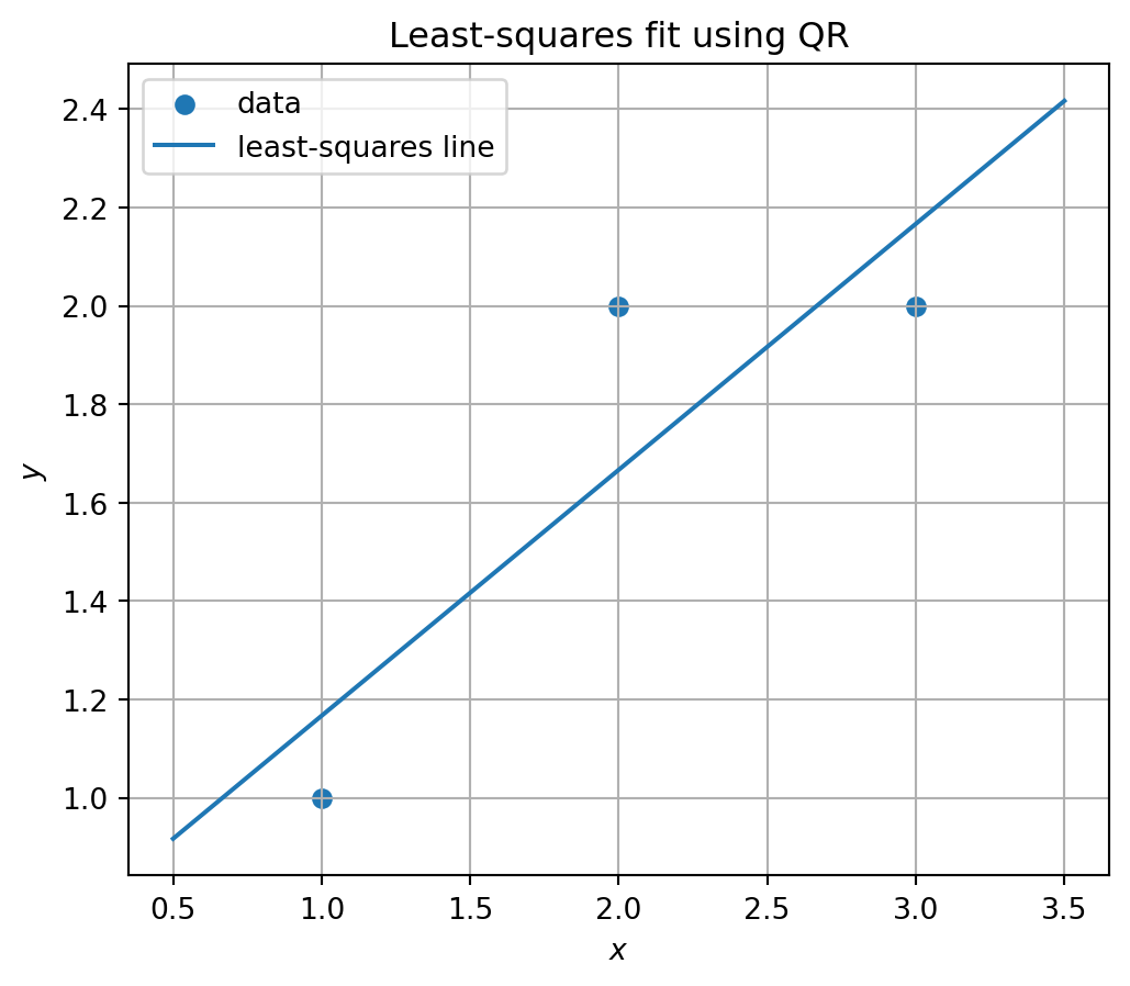
14.17 Python plot: least-squares line
= np.array([1 , 2 , 3 ], dtype= float )= np.array([1 , 2 , 2 ], dtype= float )# Design matrix for y = beta0 + beta1 x = np.column_stack([np.ones_like(x_data), x_data])= np.linalg.qr(A, mode= "reduced" )= np.linalg.solve(R, Q.T @ y_data)= np.linspace(0.5 , 3.5 , 100 )= beta[0 ] + beta[1 ] * x_grid= (6 , 5 ))= "data" )= "least-squares line" )"$x$" )"$y$" )True )"Least-squares fit using QR" )
array([0.66666667, 0.5 ])
This is an early computational view of regression.
14.18 Numerical orthogonality
In exact mathematics, Gram–Schmidt produces perfectly orthonormal vectors.
In floating-point computation, roundoff errors can accumulate.
This means that computed vectors may satisfy
\[
Q^TQ\approx I
\]
rather than exactly
\[
Q^TQ=I.
\]
The difference
\[
\|Q^TQ-I\|
\]
measures loss of orthogonality.
When vectors are nearly linearly dependent, classical Gram–Schmidt can lose orthogonality significantly.
This is why numerical linear algebra often uses modified Gram–Schmidt or Householder QR.
14.19 Classical versus modified Gram–Schmidt
The classical Gram–Schmidt formula subtracts all projections from the original vector \(a_j\) :
\[
u_j=a_j-\sum_{i=1}^{j-1}(a_j\cdot q_i)q_i.
\]
Modified Gram–Schmidt subtracts projections one at a time from the current residual vector.
The two methods are mathematically equivalent in exact arithmetic, but modified Gram–Schmidt is often more stable in finite precision.
Modified Gram–Schmidt algorithm
Start with
\[
v_j=a_j.
\]
For \(i=1,\ldots,j-1\) , compute
\[
r_{ij}=q_i^Tv_j,
\]
then update
\[
v_j\leftarrow v_j-r_{ij}q_i.
\]
Finally,
\[
r_{jj}=\|v_j\|,
\qquad
q_j=\frac{v_j}{r_{jj}}.
\]
14.20 Python: modified Gram–Schmidt
def modified_gram_schmidt(A, tol= 1e-12 ):""" Modified Gram--Schmidt for the columns of A. Returns Q and R such that A = Q R when columns are independent. """ = np.array(A, dtype= float )= A.shape= A.copy()= np.zeros((m, n))= np.zeros((n, n))for i in range (n):= np.linalg.norm(V[:, i])if R[i, i] < tol:raise ValueError ("Columns are linearly dependent or nearly dependent." )= V[:, i] / R[i, i]for j in range (i + 1 , n):= np.dot(Q[:, i], V[:, j])= V[:, j] - R[i, j] * Q[:, i]return Q, R
14.21 Python: checking numerical orthogonality
Consider a matrix with nearly dependent columns.
= 1e-8 = np.array([1 , 1 , 1 ],1 , 1 + eps, 1 ],1 , 1 , 1 + eps]= float )= gram_schmidt(A)= modified_gram_schmidt(A)= np.linalg.qr(A, mode= "reduced" )= np.linalg.norm(Q_cgs.T @ Q_cgs - np.eye(3 ))= np.linalg.norm(Q_mgs.T @ Q_mgs - np.eye(3 ))= np.linalg.norm(Q_np.T @ Q_np - np.eye(3 ))
(1.411235117099412, 1.7763568498813885e-07, 2.803986298941084e-16)
The exact numerical values may vary, but this experiment illustrates an important lesson:
Orthogonality is a numerical resource that can be lost through roundoff error.
14.22 Householder QR preview
In professional numerical linear algebra, QR factorization is often computed using Householder reflections .
A Householder reflection is an orthogonal transformation that reflects vectors across a hyperplane.
Householder QR is usually more stable than classical Gram–Schmidt.
Most numerical libraries, including NumPy and SciPy, use stable algorithms rather than the simplest classroom Gram–Schmidt algorithm.
For this course, the conceptual sequence is:
Gram–Schmidt explains the geometry.
QR factorization expresses the geometry as a matrix factorization.
Stable numerical QR implements the idea reliably.
14.23 QR and orthogonal matrices
If \(Q\) is a square matrix with orthonormal columns, then
\[
Q^TQ=I.
\]
Since \(Q\) is square, this also implies
\[
QQ^T=I.
\]
Thus
\[
Q^{-1}=Q^T.
\]
Such matrices are called orthogonal matrices .
A square matrix \(Q\) is orthogonal if
\[
Q^TQ=I.
\]
Equivalently,
\[
Q^{-1}=Q^T.
\]
Orthogonal matrices preserve lengths and dot products:
\[
\|Qx\|=\|x\|,
\]
and
\[
(Qx)\cdot(Qy)=x\cdot y.
\]
Rotations and reflections are examples of orthogonal matrices.
14.24 Python: orthogonal matrices preserve lengths
= np.pi / 5 = np.array([- np.sin(theta)],= np.array([3 , 4 ], dtype= float )@ x), Q.T @ Q
(5.0,
 5.0,
 array([[ 1.00000000e+00, -1.26599665e-17],
        [-1.26599665e-17,  1.00000000e+00]]))
The length is preserved because \(Q\) is orthogonal.
14.25 Algorithmic summary
Given independent vectors \(a_1,\ldots,a_k\) :
Set
\[
u_1=a_1,\qquad q_1=\frac{u_1}{\|u_1\|}.
\]
For \(j=2,\ldots,k\) , compute
\[
u_j=a_j-\sum_{i=1}^{j-1}(a_j\cdot q_i)q_i.
\]
Normalize:
\[
q_j=\frac{u_j}{\|u_j\|}.
\]
Given a matrix \(A\) with independent columns:
Apply Gram–Schmidt to the columns of \(A\) .
Put the orthonormal vectors into the columns of \(Q\) .
Store the coefficients in an upper triangular matrix \(R\) .
Then
\[
A=QR.
\]
If \(A=QR\) , then
\[
\operatorname{proj}_{\operatorname{Col}(A)}(b)=QQ^Tb.
\]
If \(A=QR\) has independent columns, solve
\[
R\hat x=Q^Tb.
\]
Then \(\hat x\) is the least-squares solution of \(Ax\approx b\) .
14.26 Common mistakes
Mistake 1: forgetting to subtract all previous projections
When constructing \(u_j\) , subtract the projections onto all previously computed \(q_i\) .
Mistake 2: forgetting to normalize
The vectors \(u_j\) are orthogonal, but not usually unit vectors.
The vectors \(q_j\) are orthonormal.
Mistake 3: confusing \(Q^TQ=I\) with \(QQ^T=I\)
If \(Q\) is rectangular with orthonormal columns, then
\[
Q^TQ=I.
\]
But \(QQ^T\) is usually a projection matrix, not the identity.
Mistake 4: assuming classical Gram–Schmidt is always numerically stable
Classical Gram–Schmidt explains the geometry, but it can lose orthogonality in floating-point computation.
Mistake 5: solving least squares by normal equations when QR is available
QR is usually more stable than solving
\[
A^TA\hat x=A^Tb.
\]
14.27 Chapter summary
Gram–Schmidt converts independent vectors
\[
a_1,\ldots,a_k
\]
into orthonormal vectors
\[
q_1,\ldots,q_k
\]
spanning the same subspace.
The key step is
\[
u_j=a_j-\sum_{i=1}^{j-1}(a_j\cdot q_i)q_i,
\]
followed by
\[
q_j=\frac{u_j}{\|u_j\|}.
\]
For a matrix \(A\) with independent columns, Gram–Schmidt leads to
\[
A=QR,
\]
where \(Q\) has orthonormal columns and \(R\) is upper triangular.
Projection onto \(\operatorname{Col}(A)\) can be computed as
\[
QQ^Tb.
\]
Least squares can be solved by
\[
R\hat x=Q^Tb.
\]
Numerical orthogonality matters. In floating-point computation, stable QR algorithms are essential.
Exercises
A. Gram–Schmidt by hand
Apply Gram–Schmidt to each set of vectors.
\[
a_1=
\begin{bmatrix}
1\\
1
\end{bmatrix},
\qquad
a_2=
\begin{bmatrix}
1\\
0
\end{bmatrix}.
\]
\[
a_1=
\begin{bmatrix}
1\\
0\\
1
\end{bmatrix},
\qquad
a_2=
\begin{bmatrix}
0\\
1\\
1
\end{bmatrix}.
\]
\[
a_1=
\begin{bmatrix}
1\\
1\\
0
\end{bmatrix},
\qquad
a_2=
\begin{bmatrix}
1\\
0\\
1
\end{bmatrix},
\qquad
a_3=
\begin{bmatrix}
0\\
1\\
1
\end{bmatrix}.
\]
B. QR factorization
For each matrix, find a QR factorization.
\[
A=
\begin{bmatrix}
1&1\\
1&0
\end{bmatrix}
\]
\[
A=
\begin{bmatrix}
1&0\\
1&1\\
0&1
\end{bmatrix}
\]
\[
A=
\begin{bmatrix}
1&1\\
1&2\\
1&3
\end{bmatrix}
\]
C. Projection using QR
Let
\[
A=
\begin{bmatrix}
1&1\\
1&2\\
1&3
\end{bmatrix},
\qquad
b=
\begin{bmatrix}
1\\
2\\
2
\end{bmatrix}.
\]
Compute a QR factorization of \(A\) .
Compute \(QQ^Tb\) .
Compute the error \(e=b-QQ^Tb\) .
Verify that \(A^Te=0\) .
D. Least squares using QR
Using the same \(A\) and \(b\) :
Solve
\[
R\hat x=Q^Tb.
\]
Compute \(A\hat x\) .
Compare with the projection \(QQ^Tb\) .
Interpret \(\hat x\) as coefficients of a best-fit line.
E. Orthogonal matrices
Show that the rotation matrix
\[
R_\theta=
\begin{bmatrix}
\cos\theta&-\sin\theta\\
\sin\theta&\cos\theta
\end{bmatrix}
\]
is orthogonal.
Show that if \(Q\) is orthogonal, then \(\|Qx\|=\|x\|\) .
Give an example of a reflection matrix and verify that it is orthogonal.
F. Python exercises
Implement classical Gram–Schmidt.
Implement modified Gram–Schmidt.
Compare your results with np.linalg.qr.
Check the quantity
\[
\|Q^TQ-I\|.
\]
Use QR to solve a least-squares problem.
Plot a least-squares line using QR.
Experiment with nearly dependent columns and observe loss of orthogonality.
G. Reflection
Write a short paragraph answering each question.
Why does Gram–Schmidt subtract projections?
Why is an orthonormal basis easier to use than a general basis?
What does the factorization \(A=QR\) mean geometrically?
Why is QR useful for least squares?
Why is numerical orthogonality important in computation?
AI-age connection
QR factorization is one of the workhorses of computational linear algebra. It turns unstable geometric problems into stable orthogonal computations. Least-squares regression, data fitting, numerical optimization, eigenvalue algorithms, and many scientific computing pipelines rely on QR or related orthogonal factorizations. In the age of AI, where high-dimensional data matrices are everywhere, preserving orthogonality is a way to preserve numerical reliability.