Opening question
A symmetric matrix does not only transform vectors. It also defines a geometric landscape.
Given a symmetric matrix \(A\) , the expression
\[
x^TAx
\]
assigns a number to each vector \(x\) .
For example, in two variables,
\[
x=
\begin{bmatrix}
x_1\\
x_2
\end{bmatrix},
\qquad
A=
\begin{bmatrix}
a&b\\
b&c
\end{bmatrix},
\]
we get
\[
x^TAx=ax_1^2+2bx_1x_2+cx_2^2.
\]
This is a quadratic form .
Quadratic forms describe ellipses, hyperbolas, paraboloids, energy landscapes, curvature, optimization problems, covariance geometry, and least-squares objectives.
The central question of this chapter is:
How does a symmetric matrix shape a quadratic landscape?
The answer comes from eigenvalues and eigenvectors.
Learning goals
After studying this chapter, you should be able to:
Define a quadratic form.
Write a quadratic form as \(x^TAx\) using a symmetric matrix.
Classify quadratic forms using eigenvalues.
Understand positive definite, positive semidefinite, negative definite, and indefinite matrices.
Use orthogonal diagonalization to remove cross terms.
Interpret level curves and level surfaces geometrically.
Connect quadratic forms to optimization.
Understand the Hessian matrix and curvature.
Analyze least-squares objectives as quadratic functions.
Use Python to visualize quadratic forms and optimization geometry.
20.4 Cross terms
A quadratic form may include cross terms.
For example,
\[
q(x_1,x_2)=2x_1^2+4x_1x_2+2x_2^2.
\]
This can be written as
\[
q(x)=x^TAx
\]
with
\[
A=
\begin{bmatrix}
2&2\\
2&2
\end{bmatrix}.
\]
Indeed,
\[
x^TAx
=
\begin{bmatrix}
x_1&x_2
\end{bmatrix}
\begin{bmatrix}
2&2\\
2&2
\end{bmatrix}
\begin{bmatrix}
x_1\\
x_2
\end{bmatrix}.
\]
Multiplying gives
\[
2x_1^2+4x_1x_2+2x_2^2.
\]
The off-diagonal entries split the cross term.
For a symmetric \(2\times 2\) matrix
\[
A=
\begin{bmatrix}
a&b\\
b&c
\end{bmatrix},
\]
we have
\[
x^TAx=ax_1^2+2bx_1x_2+cx_2^2.
\]
20.6 Orthogonal diagonalization removes cross terms
Let \(A\) be symmetric. By the spectral theorem,
\[
A=QDQ^T,
\]
where \(Q\) is orthogonal and \(D\) is diagonal.
Then
\[
x^TAx=x^TQDQ^Tx.
\]
Let
\[
y=Q^Tx.
\]
Since \(Q\) is orthogonal, this is a rotation or reflection of coordinates.
Then
\[
x^TAx=y^TDy.
\]
If
\[
D=\operatorname{diag}(\lambda_1,\ldots,\lambda_n),
\]
then
\[
y^TDy=\lambda_1y_1^2+\cdots+\lambda_ny_n^2.
\]
The cross terms disappear.
If \(A=QDQ^T\) and \(y=Q^Tx\) , then
\[
x^TAx=\lambda_1y_1^2+\cdots+\lambda_ny_n^2.
\]
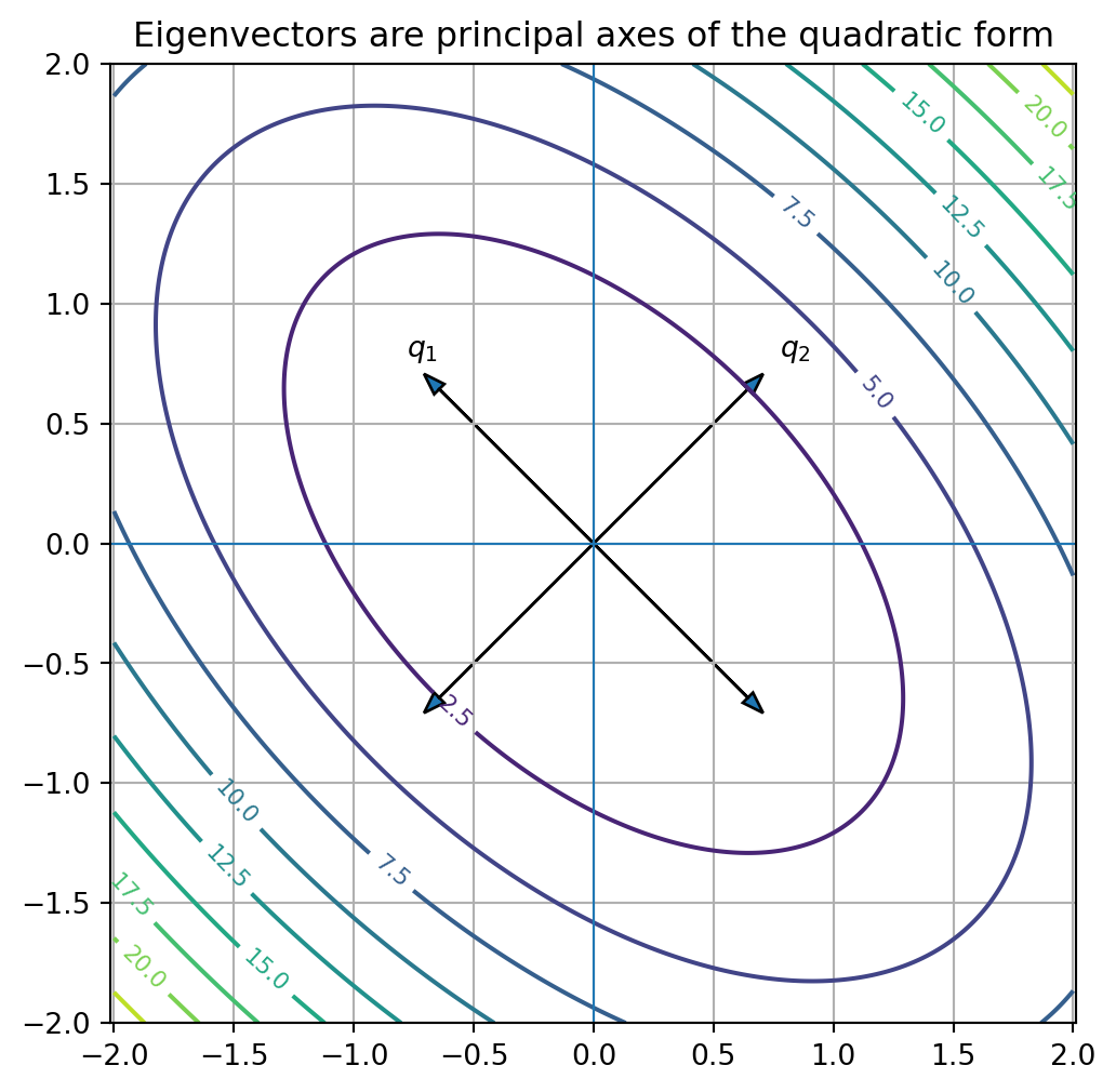
The eigenvectors give the principal axes of the quadratic form.
The eigenvalues give curvature along those axes.
20.8 Python plot: rotated ellipse
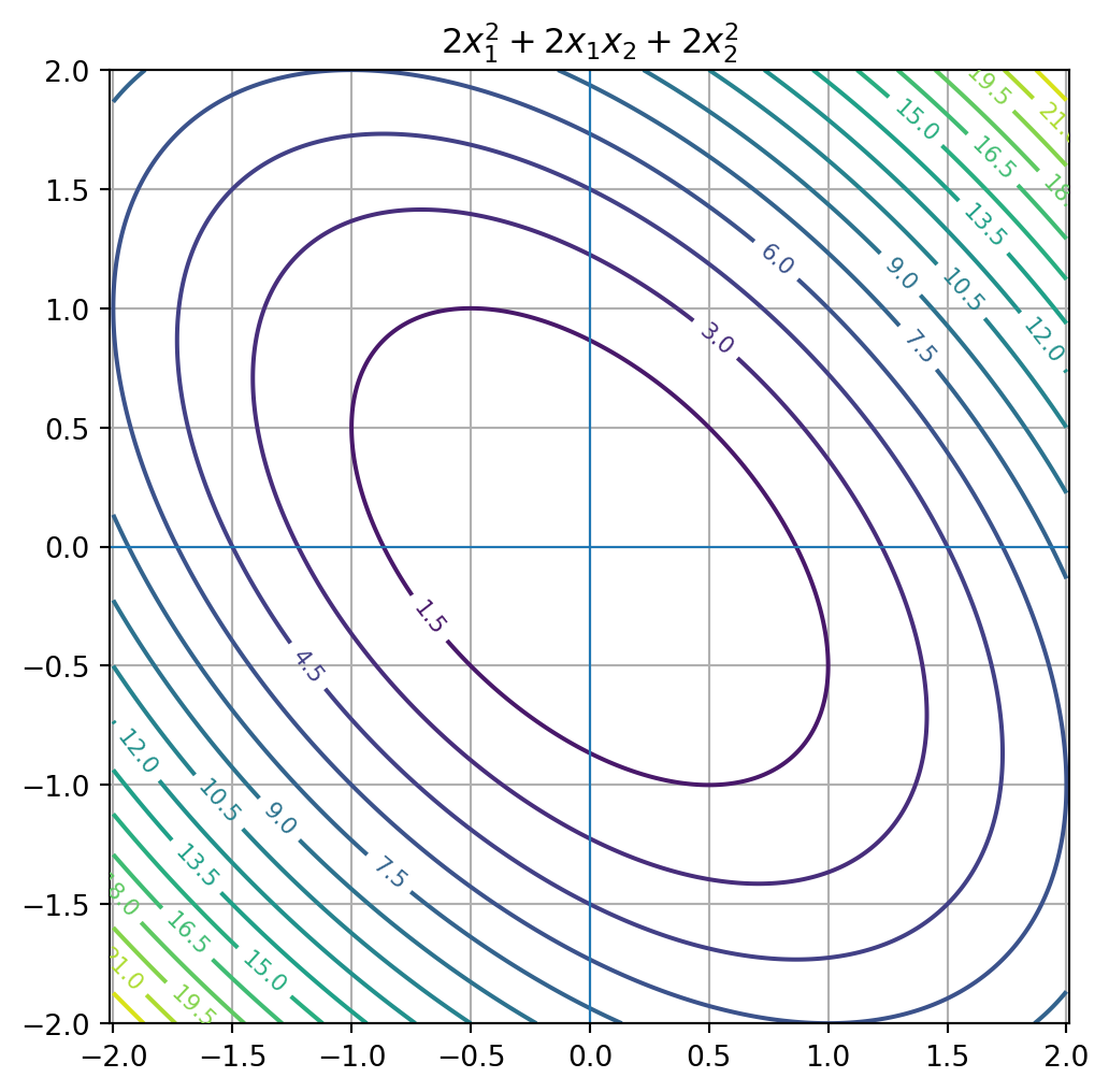
= np.array([[2 , 1 ],1 , 2 ]], dtype= float )"$2x_1^2+2x_1x_2+2x_2^2$" )
The level curves are ellipses whose axes are not aligned with the standard coordinate axes.
The eigenvectors identify the rotated principal axes.
= np.linalg.eigh(A)= (6 , 6 ))= np.linspace(- 2 , 2 , 300 )= np.linspace(- 2 , 2 , 300 )= np.meshgrid(x, y)= A[0 , 0 ]* X** 2 + 2 * A[0 , 1 ]* X* Y + A[1 , 1 ]* Y** 2 = plt.contour(X, Y, Z, levels= 10 )= True , fontsize= 8 )for j in range (2 ):= Q[:, j]0 , 0 , q[0 ], q[1 ], head_width= 0.06 , length_includes_head= True )0 , 0 , - q[0 ], - q[1 ], head_width= 0.06 , length_includes_head= True )1.1 * q[0 ], 1.1 * q[1 ], f"$q_ { j+ 1 } $" )0 , linewidth= 0.8 )0 , linewidth= 0.8 )True )"equal" )"Eigenvectors are principal axes of the quadratic form" )
(array([1., 3.]),
 array([[-0.70710678,  0.70710678],
        [ 0.70710678,  0.70710678]]))
20.9 Classification by eigenvalues
The sign of the eigenvalues determines the shape of the quadratic form.
Let \(A\) be symmetric.
Positive definite
\(A\) is positive definite if
\[
x^TAx>0
\]
for every nonzero \(x\) .
This happens exactly when all eigenvalues of \(A\) are positive.
Positive semidefinite
\(A\) is positive semidefinite if
\[
x^TAx\ge 0
\]
for every \(x\) .
This happens exactly when all eigenvalues are nonnegative.
Negative definite
\(A\) is negative definite if
\[
x^TAx<0
\]
for every nonzero \(x\) .
This happens exactly when all eigenvalues are negative.
Negative semidefinite
\(A\) is negative semidefinite if
\[
x^TAx\le 0
\]
for every \(x\) .
This happens exactly when all eigenvalues are nonpositive.
Indefinite
\(A\) is indefinite if \(x^TAx\) can be positive for some \(x\) and negative for other \(x\) .
This happens exactly when \(A\) has both positive and negative eigenvalues.
For a symmetric matrix \(A\) :
all eigenvalues positive: positive definite,
all eigenvalues nonnegative: positive semidefinite,
all eigenvalues negative: negative definite,
all eigenvalues nonpositive: negative semidefinite,
mixed positive and negative eigenvalues: indefinite.
20.10 Examples of classification
Positive definite
\[
A=
\begin{bmatrix}
4&0\\
0&1
\end{bmatrix}
\]
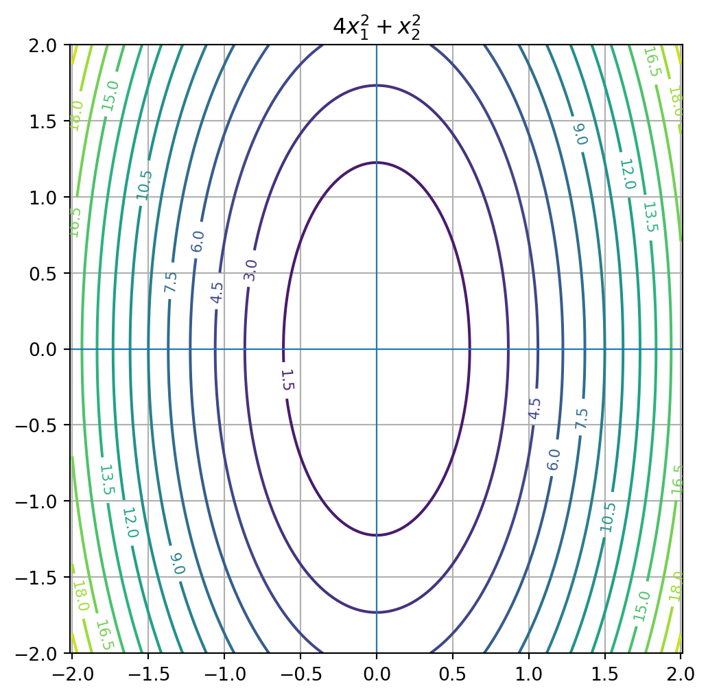
has eigenvalues \(4\) and \(1\) .
Both are positive, so \(A\) is positive definite.
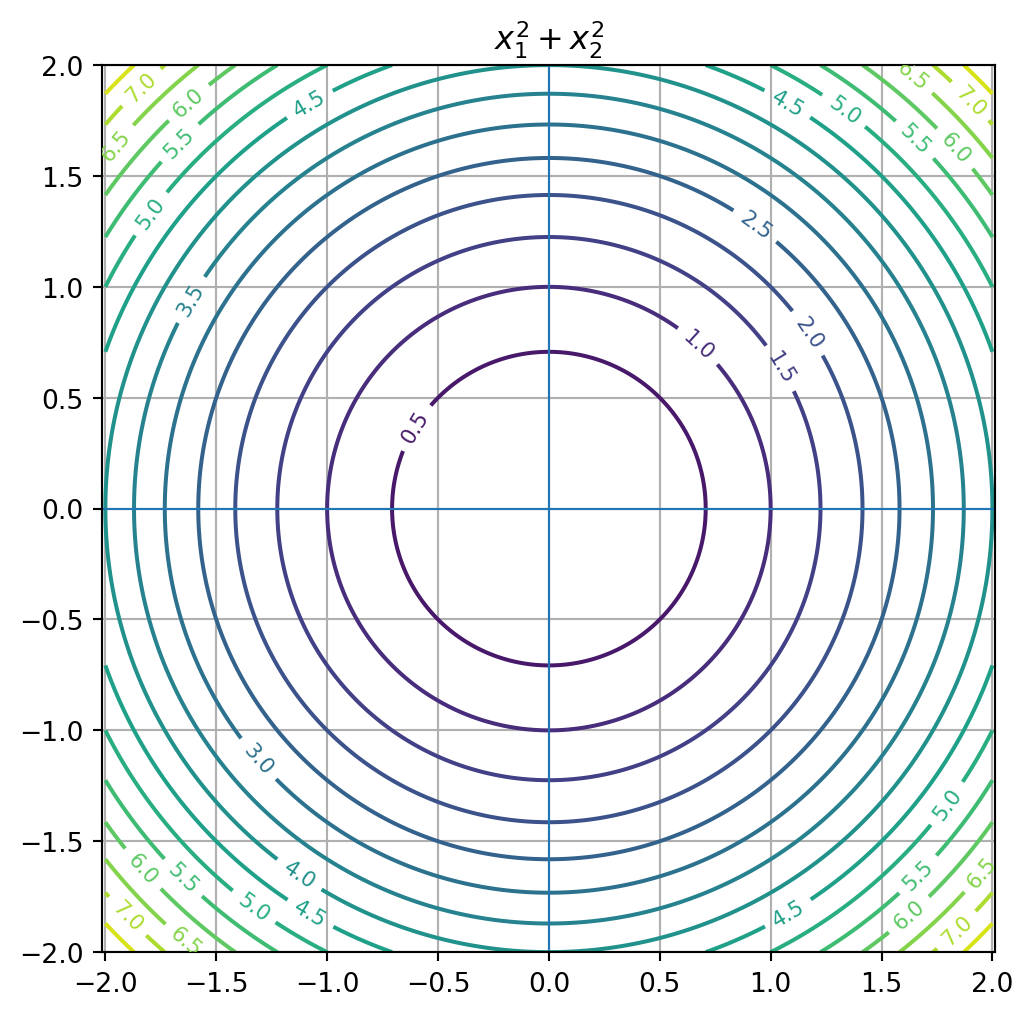
The level curves are ellipses.
Positive semidefinite
\[
A=
\begin{bmatrix}
1&0\\
0&0
\end{bmatrix}
\]
has eigenvalues \(1\) and \(0\) .
It is positive semidefinite, but not positive definite.
The quadratic form is
\[
x_1^2.
\]
It is zero for all vectors on the \(x_2\) -axis.
Indefinite
\[
A=
\begin{bmatrix}
1&0\\
0&-1
\end{bmatrix}
\]
has eigenvalues \(1\) and \(-1\) .
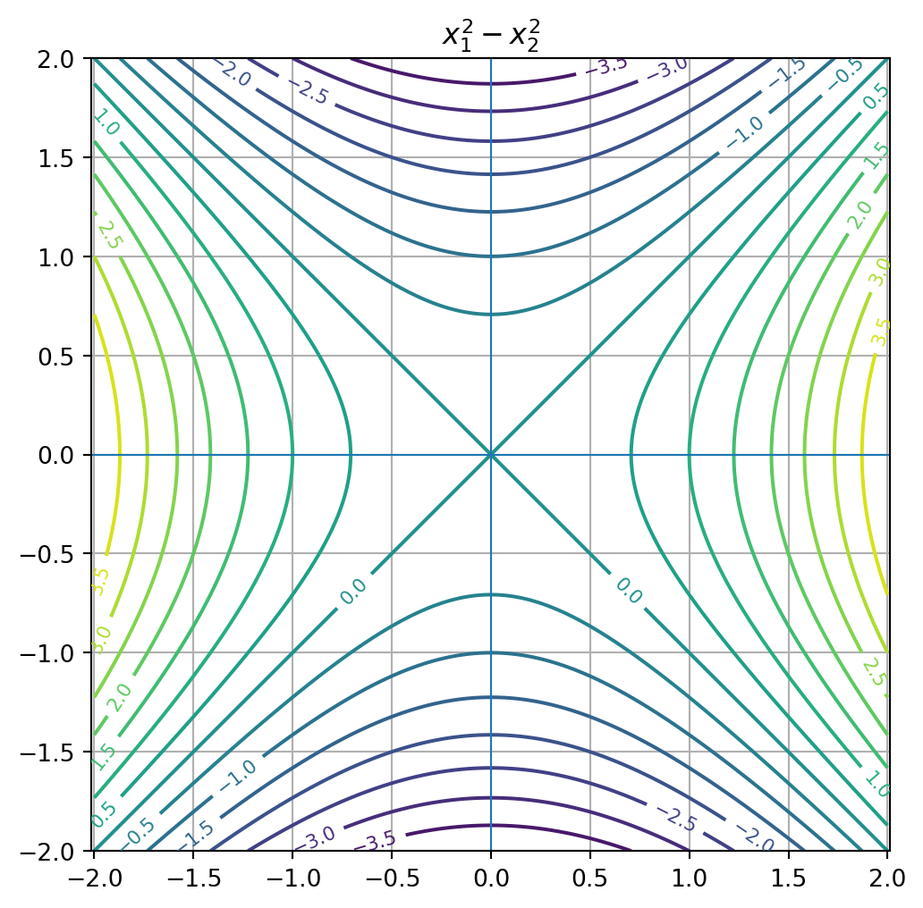
It is indefinite.
The quadratic form is
\[
x_1^2-x_2^2.
\]
It can be positive, negative, or zero.
20.11 Python: classification by eigenvalues
def classify_symmetric(A, tol= 1e-10 ):= np.linalg.eigvalsh(A)if np.all (eigvals > tol):= "positive definite" elif np.all (eigvals >= - tol) and np.any (np.abs (eigvals) <= tol):= "positive semidefinite" elif np.all (eigvals < - tol):= "negative definite" elif np.all (eigvals <= tol) and np.any (np.abs (eigvals) <= tol):= "negative semidefinite" elif np.any (eigvals > tol) and np.any (eigvals < - tol):= "indefinite" else := "borderline / numerical ambiguity" return eigvals, kind= {"positive definite" : np.array([[4 , 0 ], [0 , 1 ]], dtype= float ),"positive semidefinite" : np.array([[1 , 0 ], [0 , 0 ]], dtype= float ),"indefinite" : np.array([[1 , 0 ], [0 , - 1 ]], dtype= float ),"rotated positive definite" : np.array([[2 , 1 ], [1 , 2 ]], dtype= float )for name, A in matrices.items():= classify_symmetric(A)print (name)print ("eigenvalues:" , eigvals)print ("classification:" , kind)print ()
positive definite
eigenvalues: [1. 4.]
classification: positive definite

positive semidefinite
eigenvalues: [0. 1.]
classification: positive semidefinite

indefinite
eigenvalues: [-1.  1.]
classification: indefinite

rotated positive definite
eigenvalues: [1. 3.]
classification: positive definite
20.12 Positive definite matrices and ellipses
If \(A\) is positive definite, then
\[
x^TAx=c
\]
for \(c>0\) is an ellipse in \(\mathbb{R}^2\) or an ellipsoid in higher dimensions.
Using the spectral theorem,
\[
x^TAx=\lambda_1y_1^2+\lambda_2y_2^2.
\]
For \(c=1\) ,
\[
\lambda_1y_1^2+\lambda_2y_2^2=1.
\]
This can be written as
\[
\frac{y_1^2}{1/\lambda_1}+\frac{y_2^2}{1/\lambda_2}=1.
\]
So the axis lengths are
\[
\frac{1}{\sqrt{\lambda_1}}
\quad \text{and} \quad
\frac{1}{\sqrt{\lambda_2}}.
\]
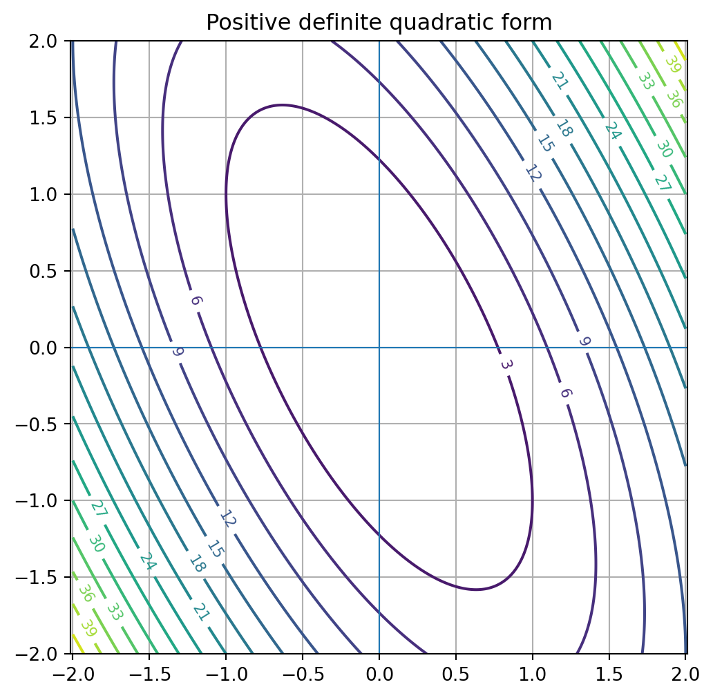
Large eigenvalues correspond to short axes and steep curvature.
Small eigenvalues correspond to long axes and shallow curvature.
20.13 Python plot: eigenvalues and ellipse axes
= np.array([[5 , 2 ],2 , 2 ]], dtype= float )= np.linalg.eigh(A)"Positive definite quadratic form" )print ("eigenvalues:" , eigvals)print ("axis lengths for level x^T A x = 1:" , 1 / np.sqrt(eigvals))
eigenvalues: [1. 6.]
axis lengths for level x^T A x = 1: [1.         0.40824829]
The eigenvectors give directions of the ellipse axes.
The eigenvalues determine the inverse squared axis lengths.
20.14 Sylvester’s criterion for \(2\times 2\) matrices
For a symmetric \(2\times 2\) matrix
\[
A=
\begin{bmatrix}
a&b\\
b&c
\end{bmatrix},
\]
there is a useful test for positive definiteness.
The matrix is positive definite if and only if
\[
a>0
\]
and
\[
\det(A)>0.
\]
For
\[
A=
\begin{bmatrix}
a&b\\
b&c
\end{bmatrix},
\]
\(A\) is positive definite if and only if
\[
a>0
\quad \text{and} \quad
\det(A)>0.
\]
This is a special case of Sylvester’s criterion.
For larger symmetric matrices, positive definiteness can be tested using leading principal minors or eigenvalues.
20.15 Optimization and quadratic functions
A quadratic function has the form
\[
f(x)=\frac12 x^TAx-b^Tx+c,
\]
where \(A\) is symmetric.
The gradient is
\[
\nabla f(x)=Ax-b.
\]
The Hessian matrix is
\[
\nabla^2 f(x)=A.
\]
Thus the symmetric matrix \(A\) controls the curvature of the function.
Critical points satisfy
\[
\nabla f(x)=0.
\]
So
\[
Ax=b.
\]
If \(A\) is positive definite, then the critical point is the unique global minimum.
If \(A\) is positive definite, then
\[
f(x)=\frac12x^TAx-b^Tx+c
\]
has a unique global minimum at the solution of
\[
Ax=b.
\]
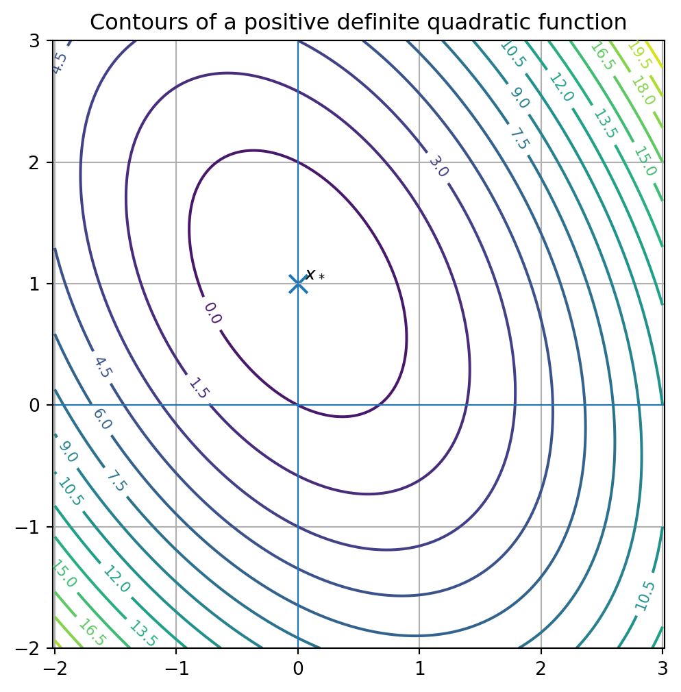
20.17 Python plot: quadratic bowl
= np.array([[3 , 1 ],1 , 2 ]], dtype= float )= np.array([1 , 2 ], dtype= float )= np.linalg.solve(A, b)= np.linspace(- 2 , 3 , 250 )= np.linspace(- 2 , 3 , 250 )= np.meshgrid(x, y)= (0.5 * (A[0 , 0 ]* X** 2 + 2 * A[0 , 1 ]* X* Y + A[1 , 1 ]* Y** 2 )- b[0 ]* X - b[1 ]* Y= (6 , 6 ))= plt.contour(X, Y, Z, levels= 20 )= True , fontsize= 8 )0 ]], [x_star[1 ]], marker= "x" , s= 100 )0 ] + 0.05 , x_star[1 ] + 0.05 , "$x_*$" )0 , linewidth= 0.8 )0 , linewidth= 0.8 )True )"equal" )"Contours of a positive definite quadratic function" )
The point \(x_*\) is the unique minimizer.
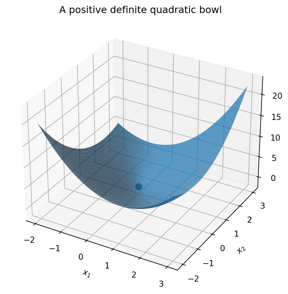
20.18 Three-dimensional surface plot
= plt.figure(figsize= (8 , 6 ))= fig.add_subplot(111 , projection= "3d" )= 0.75 , linewidth= 0 )0 ]], [x_star[1 ]], [0.5 * x_star @ A @ x_star - b @ x_star], s= 60 )"$x_1$" )"$x_2$" )"$f(x)$" )"A positive definite quadratic bowl" )
A positive definite quadratic function is shaped like a bowl.
A negative definite quadratic function is shaped like an upside-down bowl.
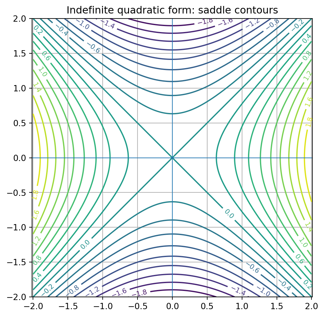
An indefinite quadratic function is shaped like a saddle.
20.19 Indefinite quadratic functions and saddles
Let
\[
A=
\begin{bmatrix}
1&0\\
0&-1
\end{bmatrix}.
\]
Then
\[
f(x)=\frac12x^TAx=\frac12(x_1^2-x_2^2).
\]
Along the \(x_1\) direction, the function increases.
Along the \(x_2\) direction, the function decreases.
So the origin is a saddle point, not a minimum or maximum.
= np.array([[1 , 0 ],0 , - 1 ]], dtype= float )= np.linspace(- 2 , 2 , 250 )= np.linspace(- 2 , 2 , 250 )= np.meshgrid(x, y)= 0.5 * (X** 2 - Y** 2 )= (6 , 6 ))= plt.contour(X, Y, Z, levels= 20 )= True , fontsize= 8 )0 , linewidth= 0.8 )0 , linewidth= 0.8 )True )"equal" )"Indefinite quadratic form: saddle contours" )
20.20 Hessian matrix and local optimization
For a twice differentiable function \(f:\mathbb{R}^n\to\mathbb{R}\) , the Hessian matrix is
\[
H(x)=
\begin{bmatrix}
\frac{\partial^2 f}{\partial x_1^2}&\cdots&\frac{\partial^2 f}{\partial x_1\partial x_n}\\
\vdots&\ddots&\vdots\\
\frac{\partial^2 f}{\partial x_n\partial x_1}&\cdots&\frac{\partial^2 f}{\partial x_n^2}
\end{bmatrix}.
\]
Near a critical point \(x_*\) , a function can be approximated by a quadratic model:
\[
f(x_*+h)\approx f(x_*)+\frac12 h^TH(x_*)h.
\]
Thus the eigenvalues of the Hessian determine local shape:
all positive eigenvalues: local minimum,
all negative eigenvalues: local maximum,
mixed signs: saddle point.
This is the second derivative test in multivariable form.
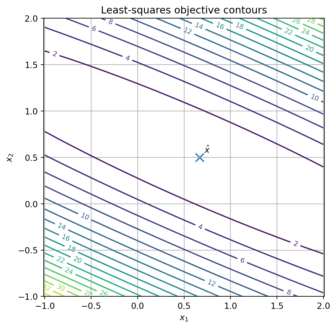
20.22 Python plot: least-squares objective surface
= np.array([1 , 1 ],1 , 2 ],1 , 3 ]= float )= np.array([1 , 2 , 2 ], dtype= float )= np.linalg.lstsq(A, b, rcond= None )[0 ]= np.linspace(- 1 , 2 , 200 )= np.linspace(- 1 , 2 , 200 )= np.meshgrid(u, v)= np.zeros_like(U)for i in range (U.shape[0 ]):for j in range (U.shape[1 ]):= np.array([U[i, j], V[i, j]])= 0.5 * np.linalg.norm(A @ x_vec - b)** 2 = (6 , 6 ))= plt.contour(U, V, Z, levels= 20 )= True , fontsize= 8 )0 ]], [x_star[1 ]], marker= "x" , s= 100 )0 ] + 0.05 , x_star[1 ] + 0.05 , "$ \\ hat x$" )"$x_1$" )"$x_2$" )True )"equal" )"Least-squares objective contours" )
array([0.66666667, 0.5 ])
20.23 Gradient descent on a quadratic
For
\[
f(x)=\frac12x^TAx-b^Tx,
\]
where \(A\) is positive definite, gradient descent is
\[
x_{k+1}=x_k-\alpha(Ax_k-b).
\]
The error
\[
e_k=x_k-x_*
\]
satisfies
\[
e_{k+1}=(I-\alpha A)e_k.
\]
Therefore convergence depends on eigenvalues of
\[
I-\alpha A.
\]
If \(A\) has eigenvalues \(\lambda_i\) , then \(I-\alpha A\) has eigenvalues
\[
1-\alpha\lambda_i.
\]
For convergence, we need
\[
|1-\alpha\lambda_i|<1
\]
for all \(i\) .
This gives
\[
0<\alpha<\frac{2}{\lambda_{\max}}.
\]
Eigenvalues determine the allowed step size.
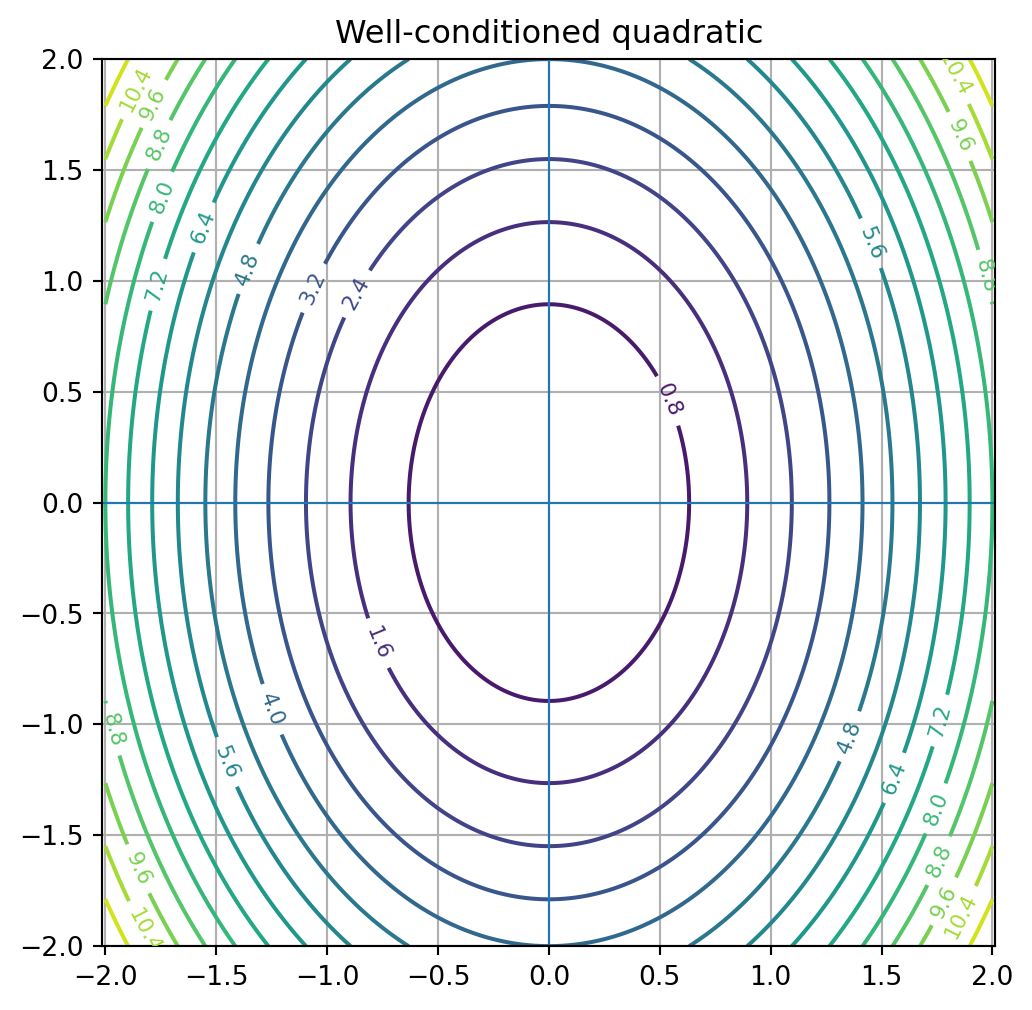
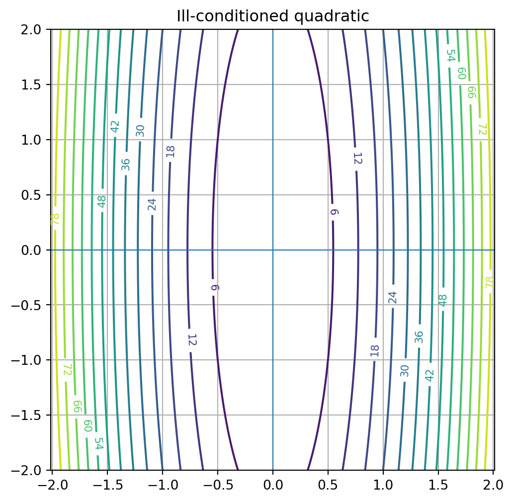
20.24 Conditioning and elongated contours
If \(A\) is positive definite, its condition number is
\[
\kappa(A)=\frac{\lambda_{\max}}{\lambda_{\min}}.
\]
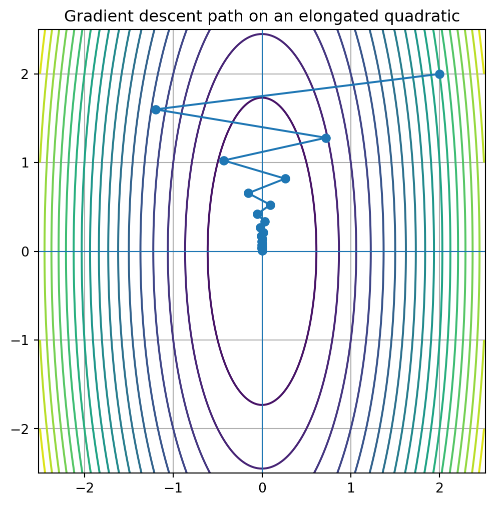
When \(\kappa(A)\) is large, level curves are highly elongated.
Gradient descent may zigzag and converge slowly.
This is a key reason eigenvalues matter in optimization.
= np.array([[2 , 0 ],0 , 1 ]], dtype= float )= np.array([[20 , 0 ],0 , 1 ]], dtype= float )"Well-conditioned quadratic" )"Ill-conditioned quadratic" )
20.25 Python: gradient descent paths
def gradient_descent_quadratic(A, b, x0, alpha, steps):= x0.astype(float ).copy()= [x.copy()]for _ in range (steps):= A @ x - b= x - alpha * gradreturn np.array(path)= np.array([[8 , 0 ],0 , 1 ]], dtype= float )= np.array([0 , 0 ], dtype= float )= gradient_descent_quadratic(= A,= b,= np.array([2.0 , 2.0 ]),= 0.20 ,= 25 = np.linspace(- 2.5 , 2.5 , 250 )= np.linspace(- 2.5 , 2.5 , 250 )= np.meshgrid(x, y)= 0.5 * (A[0 ,0 ]* X** 2 + A[1 ,1 ]* Y** 2 )= (6 , 6 ))= plt.contour(X, Y, Z, levels= 20 )0 ], path[:, 1 ], marker= "o" )0 , linewidth= 0.8 )0 , linewidth= 0.8 )True )"equal" )"Gradient descent path on an elongated quadratic" )
20.27 Mahalanobis distance preview
If \(A\) is positive definite, then
\[
\|x\|_A=\sqrt{x^TAx}
\]
defines a geometry-dependent length.
The corresponding distance is
\[
d_A(x,y)=\sqrt{(x-y)^TA(x-y)}.
\]
When \(A=C^{-1}\) for a covariance matrix \(C\) , this is called the Mahalanobis distance .
It measures distance while accounting for different scales and correlations in the data.
Level sets of Mahalanobis distance are ellipses aligned with covariance eigenvectors.
20.28 Algorithmic summary
For a quadratic form:
Put squared-term coefficients on the diagonal.
Split each cross-term coefficient equally across symmetric off-diagonal entries.
Use a symmetric matrix \(A\) so that
\[
q(x)=x^TAx.
\]
Given a symmetric matrix \(A\) :
Compute its eigenvalues.
If all are positive, \(A\) is positive definite.
If all are nonnegative, \(A\) is positive semidefinite.
If all are negative, \(A\) is negative definite.
If all are nonpositive, \(A\) is negative semidefinite.
If signs are mixed, \(A\) is indefinite.
Given a symmetric matrix \(A\) :
Orthogonally diagonalize
\[
A=QDQ^T.
\]
Change variables using
\[
y=Q^Tx.
\]
Then
\[
x^TAx=y^TDy.
\]
For
\[
f(x)=\frac12x^TAx-b^Tx+c
\]
with \(A\) positive definite:
Solve
\[
Ax=b.
\]
The solution
\[
x_*=A^{-1}b
\]
is the unique global minimizer.
20.29 Common mistakes
Mistake 1: forgetting to split cross terms
The quadratic form
\[
4x_1x_2
\]
corresponds to off-diagonal entries \(2\) and \(2\) , not \(4\) and \(4\) .
Mistake 2: using a nonsymmetric matrix unnecessarily
Quadratic forms should be represented by symmetric matrices.
The skew-symmetric part contributes nothing to \(x^TAx\) .
Mistake 3: confusing positive entries with positive definiteness
A matrix with positive entries is not necessarily positive definite.
Positive definiteness depends on eigenvalues or equivalent tests.
Mistake 5: assuming every critical point is a minimum
If the Hessian is indefinite, the critical point is a saddle.
Mistake 6: ignoring conditioning
A positive definite quadratic can still be hard to optimize if its eigenvalues are very uneven.
20.30 Chapter summary
A quadratic form has the form
\[
q(x)=x^TAx,
\]
where \(A\) is symmetric.
For
\[
A=
\begin{bmatrix}
a&b\\
b&c
\end{bmatrix},
\]
we have
\[
x^TAx=ax_1^2+2bx_1x_2+cx_2^2.
\]
By the spectral theorem,
\[
A=QDQ^T.
\]
With
\[
y=Q^Tx,
\]
the quadratic form becomes
\[
x^TAx=y^TDy=\lambda_1y_1^2+\cdots+\lambda_ny_n^2.
\]
Eigenvalues classify the quadratic form.
Positive definite matrices produce bowls and ellipses.
Indefinite matrices produce saddles and hyperbolas.
For a quadratic function
\[
f(x)=\frac12x^TAx-b^Tx+c,
\]
the gradient is
\[
\nabla f(x)=Ax-b.
\]
If \(A\) is positive definite, the unique minimizer solves
\[
Ax=b.
\]
Least squares is a quadratic optimization problem with Hessian \(A^TA\) .
Quadratic forms connect geometry, optimization, covariance, PCA, and machine learning.
Exercises
B. Classification
Classify each symmetric matrix as positive definite, positive semidefinite, negative definite, negative semidefinite, or indefinite.
\[
\begin{bmatrix}
4&0\\
0&1
\end{bmatrix}
\]
\[
\begin{bmatrix}
1&0\\
0&0
\end{bmatrix}
\]
\[
\begin{bmatrix}
1&0\\
0&-1
\end{bmatrix}
\]
\[
\begin{bmatrix}
2&1\\
1&2
\end{bmatrix}
\]
\[
\begin{bmatrix}
1&2\\
2&1
\end{bmatrix}
\]
C. Principal axes
For
\[
A=
\begin{bmatrix}
2&1\\
1&2
\end{bmatrix},
\]
Find eigenvalues and orthonormal eigenvectors.
Form \(Q\) and \(D\) .
Verify that \(A=QDQ^T\) .
Write \(x^TAx\) in the coordinates \(y=Q^Tx\) .
D. Optimization
For each quadratic function, find the critical point and classify it.
\[
f(x)=\frac12x^T
\begin{bmatrix}
2&0\\
0&4
\end{bmatrix}
x-
\begin{bmatrix}
2\\
8
\end{bmatrix}^Tx
\]
\[
f(x)=\frac12x^T
\begin{bmatrix}
1&0\\
0&-1
\end{bmatrix}
x
\]
\[
f(x)=\frac12x^T
\begin{bmatrix}
3&1\\
1&2
\end{bmatrix}
x-
\begin{bmatrix}
1\\
2
\end{bmatrix}^Tx
\]
E. Least squares as quadratic optimization
Let
\[
A=
\begin{bmatrix}
1&1\\
1&2\\
1&3
\end{bmatrix},
\qquad
b=
\begin{bmatrix}
1\\
2\\
2
\end{bmatrix}.
\]
Write
\[
f(x)=\frac12\|Ax-b\|^2
\]
in the form
\[
\frac12x^THx-g^Tx+c.
\]
Identify \(H\) and \(g\) .
Solve \(Hx=g\) .
Compare with the least-squares solution.
F. Gradient descent
For
\[
f(x)=\frac12x^TAx
\]
with
\[
A=
\begin{bmatrix}
8&0\\
0&1
\end{bmatrix},
\]
Find the eigenvalues of \(A\) .
Determine a range of step sizes \(\alpha\) for convergence.
Run gradient descent from \(x_0=(2,2)\) .
Plot the path over contour curves.
G. Python exercises
Write a function that plots level curves of a \(2\times 2\) quadratic form.
Write a function that classifies a symmetric matrix by eigenvalues.
Generate positive definite matrices and plot their ellipses.
Generate indefinite matrices and plot their saddle contours.
Visualize gradient descent on well-conditioned and ill-conditioned quadratics.
Compute the covariance matrix of a data set and plot its principal axes.
Explore how eigenvalues affect ellipse shape.
H. Reflection
Write a short paragraph answering each question.
Why do symmetric matrices naturally define quadratic forms?
Why do eigenvectors give principal axes?
Why do positive eigenvalues create bowls and ellipses?
Why do mixed eigenvalue signs create saddle geometry?
How do quadratic forms connect linear algebra to optimization and AI?
AI-age connection
Quadratic forms are the local geometry of optimization. Near a minimum, many complicated loss functions look approximately quadratic, and the Hessian determines curvature. In least squares, the entire objective is quadratic. In machine learning, eigenvalues of curvature matrices influence conditioning, convergence speed, and stability. Covariance matrices and PCA use positive semidefinite quadratic geometry to identify principal directions of data. Quadratic forms are therefore a bridge from linear algebra to optimization, statistics, and AI.