18 Determinants and Volume

18.1 Opening question

A square matrix transforms space.

It may stretch, shrink, shear, reflect, rotate, or collapse.

One number measures how a matrix changes signed volume.

That number is the determinant.

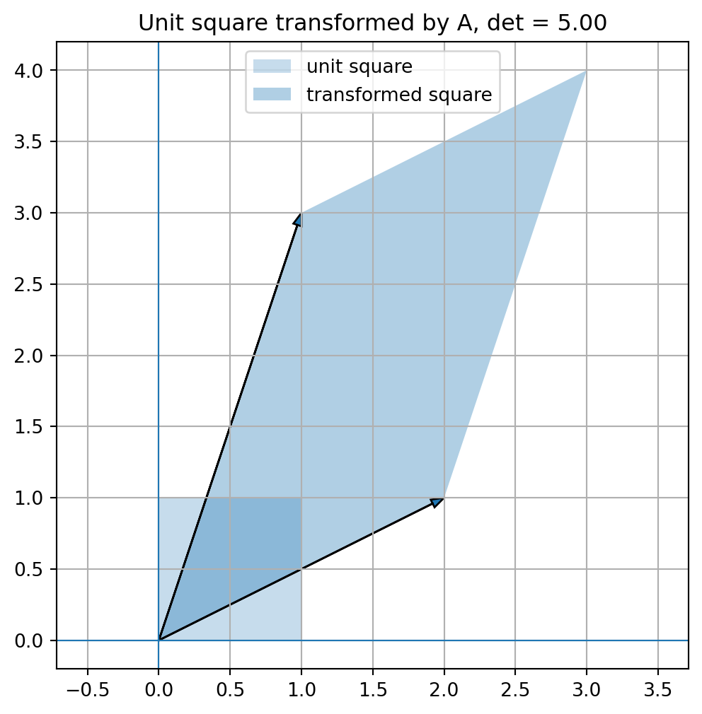
For a \(2\times 2\) matrix, the determinant measures signed area scaling.

For a \(3\times 3\) matrix, it measures signed volume scaling.

For an \(n\times n\) matrix, it measures signed \(n\)-dimensional volume scaling.

The determinant answers several important questions at once:

Does a matrix collapse space?
Is a square matrix invertible?
How does a linear transformation change area or volume?
Does a transformation preserve or reverse orientation?
What is the volume of a parallelogram, parallelepiped, or higher-dimensional box?

The central question of this chapter is:

How does a matrix scale volume?

18.2 Learning goals

After studying this chapter, you should be able to:

Compute determinants of \(2\times 2\) and \(3\times 3\) matrices.
Interpret determinants geometrically as signed area or volume scaling.
Use determinants to test invertibility.
Understand how row operations affect determinants.
Compute determinants using row reduction.
Use determinant properties to simplify calculations.
Understand orientation and sign of determinant.
Relate determinant zero to linear dependence.
Use determinants to compute areas and volumes.
Use Python to visualize determinant geometry and compute determinants.

18.3 16.1 Determinant of a \(2\times 2\) matrix

For a \(2\times 2\) matrix

\[ A= \begin{bmatrix} a&b\\ c&d \end{bmatrix}, \]

the determinant is

\[ \det(A)=ad-bc. \]

Definition: determinant of a \(2\times 2\) matrix

\[ \det \begin{bmatrix} a&b\\ c&d \end{bmatrix} = ad-bc. \]

18.3.1 Example

Let

\[ A= \begin{bmatrix} 1&2\\ 3&4 \end{bmatrix}. \]

Then

\[ \det(A)=1(4)-2(3)=4-6=-2. \]

The determinant is negative, so the transformation reverses orientation.

Its absolute value is \(2\), so the transformation scales area by a factor of \(2\).

18.4 16.2 Determinant and area in \(\mathbb{R}^2\)

Let

\[ A= \begin{bmatrix} |&|\\ a_1&a_2\\ |&| \end{bmatrix} \]

be a \(2\times 2\) matrix with columns \(a_1\) and \(a_2\).

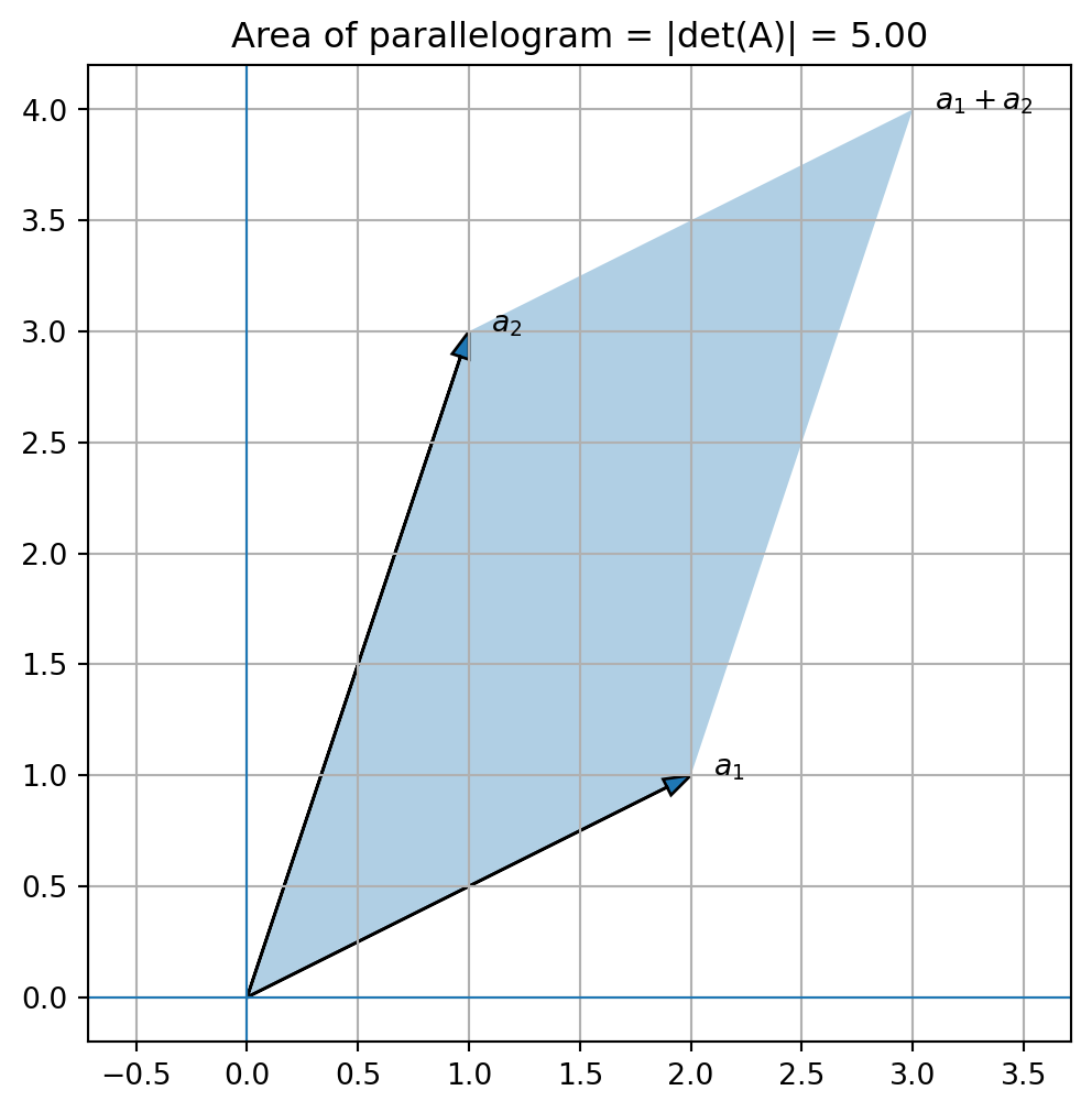
The columns \(a_1\) and \(a_2\) form a parallelogram.

The area of this parallelogram is

\[ |\det(A)|. \]

Area interpretation

For a \(2\times 2\) matrix \(A\),

\[ |\det(A)| \]

is the area of the parallelogram formed by the columns of \(A\).

The sign of the determinant tells whether orientation is preserved or reversed.

If \(\det(A)>0\), orientation is preserved.
If \(\det(A)<0\), orientation is reversed.
If \(\det(A)=0\), the parallelogram has zero area.

18.5 16.3 Python plot: determinant as area

import numpy as np
import matplotlib.pyplot as plt
from matplotlib.patches import Polygon

A = np.array([[2, 1],
              [1, 3]], dtype=float)

a1 = A[:, 0]
a2 = A[:, 1]

parallelogram = np.array([
    [0, 0],
    a1,
    a1 + a2,
    a2
])

detA = np.linalg.det(A)

plt.figure(figsize=(6, 6))
poly = Polygon(parallelogram, closed=True, alpha=0.35)
plt.gca().add_patch(poly)

plt.arrow(0, 0, a1[0], a1[1], head_width=0.08, length_includes_head=True)
plt.arrow(0, 0, a2[0], a2[1], head_width=0.08, length_includes_head=True)

plt.text(a1[0] + 0.1, a1[1], "$a_1$")
plt.text(a2[0] + 0.1, a2[1], "$a_2$")
plt.text((a1+a2)[0] + 0.1, (a1+a2)[1], "$a_1+a_2$")
plt.axhline(0, linewidth=0.8)
plt.axvline(0, linewidth=0.8)
plt.grid(True)
plt.axis("equal")
plt.title(f"Area of parallelogram = |det(A)| = {abs(detA):.2f}")
plt.show()

18.6 16.4 Determinant zero means collapse

Consider

\[ A= \begin{bmatrix} 1&2\\ 2&4 \end{bmatrix}. \]

Then

\[ \det(A)=1(4)-2(2)=0. \]

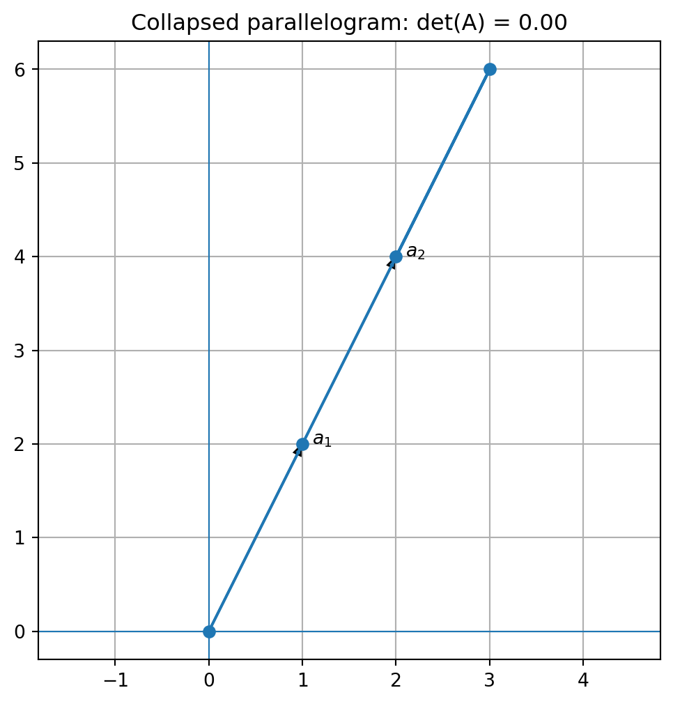
The columns are

\[ a_1= \begin{bmatrix} 1\\ 2 \end{bmatrix}, \qquad a_2= \begin{bmatrix} 2\\ 4 \end{bmatrix}. \]

Since

\[ a_2=2a_1, \]

the columns lie on the same line.

The parallelogram formed by the columns has zero area.

The matrix collapses the plane onto a line.

Thus the transformation is not invertible.

Determinant zero

For a square matrix \(A\),

\[ \det(A)=0 \]

means that \(A\) collapses volume and is not invertible.

18.7 16.5 Python plot: zero determinant collapse

A = np.array([[1, 2],
              [2, 4]], dtype=float)

a1 = A[:, 0]
a2 = A[:, 1]

parallelogram = np.array([
    [0, 0],
    a1,
    a1 + a2,
    a2
])

detA = np.linalg.det(A)

plt.figure(figsize=(6, 6))
plt.plot(parallelogram[:, 0], parallelogram[:, 1], marker="o")
plt.arrow(0, 0, a1[0], a1[1], head_width=0.08, length_includes_head=True)
plt.arrow(0, 0, a2[0], a2[1], head_width=0.08, length_includes_head=True)
plt.text(a1[0] + 0.1, a1[1], "$a_1$")
plt.text(a2[0] + 0.1, a2[1], "$a_2$")
plt.axhline(0, linewidth=0.8)
plt.axvline(0, linewidth=0.8)
plt.grid(True)
plt.axis("equal")
plt.title(f"Collapsed parallelogram: det(A) = {detA:.2f}")
plt.show()

18.8 16.6 Determinant and orientation

The sign of a determinant records orientation.

In \(\mathbb{R}^2\), the standard ordered basis

\[ e_1= \begin{bmatrix} 1\\ 0 \end{bmatrix}, \qquad e_2= \begin{bmatrix} 0\\ 1 \end{bmatrix} \]

has positive orientation.

If a matrix sends \(e_1,e_2\) to columns \(a_1,a_2\) that keep the same counterclockwise orientation, then

\[ \det(A)>0. \]

If the transformation flips orientation, then

\[ \det(A)<0. \]

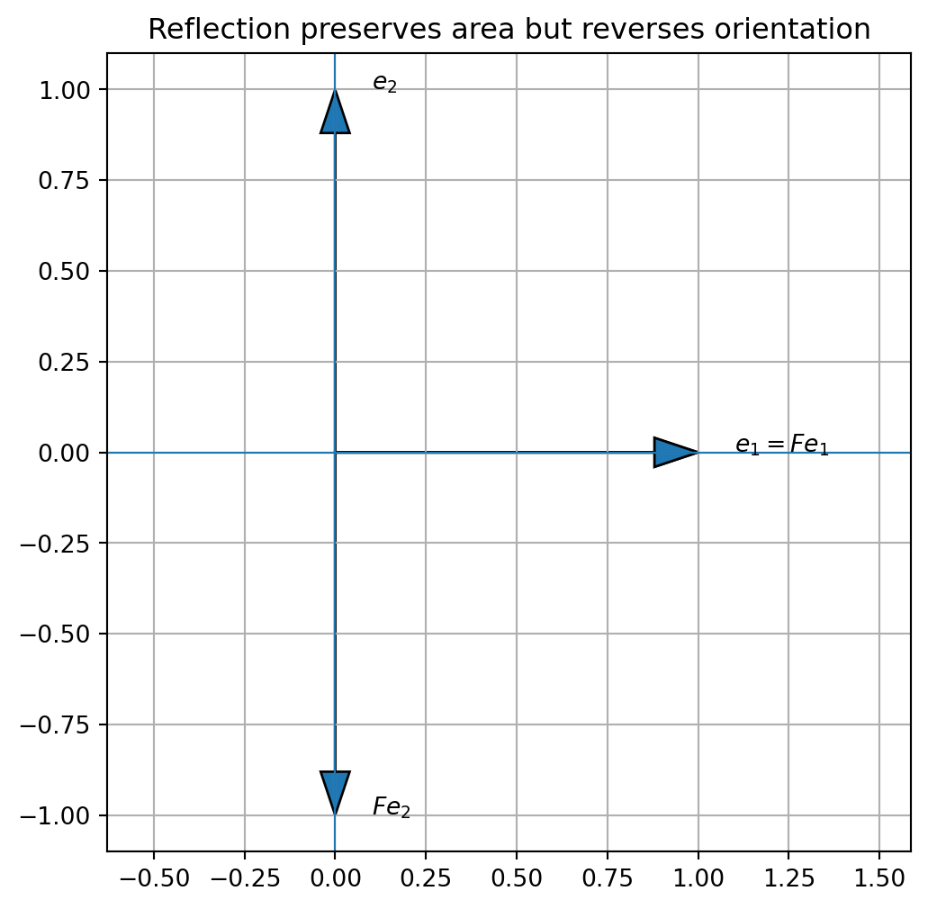
For example,

\[ F= \begin{bmatrix} 1&0\\ 0&-1 \end{bmatrix} \]

reflects across the \(x\)-axis.

Its determinant is

\[ \det(F)=-1. \]

The absolute value is \(1\), so areas are preserved.

The negative sign indicates orientation reversal.

18.9 16.7 Python plot: orientation reversal

F = np.array([[1, 0],
              [0, -1]], dtype=float)

e1 = np.array([1, 0])
e2 = np.array([0, 1])
Fe1 = F @ e1
Fe2 = F @ e2

plt.figure(figsize=(6, 6))
plt.arrow(0, 0, e1[0], e1[1], head_width=0.08, length_includes_head=True)
plt.arrow(0, 0, e2[0], e2[1], head_width=0.08, length_includes_head=True)
plt.arrow(0, 0, Fe1[0], Fe1[1], head_width=0.08, length_includes_head=True)
plt.arrow(0, 0, Fe2[0], Fe2[1], head_width=0.08, length_includes_head=True)
plt.text(e1[0] + 0.1, e1[1], "$e_1=Fe_1$")
plt.text(e2[0] + 0.1, e2[1], "$e_2$")
plt.text(Fe2[0] + 0.1, Fe2[1], "$Fe_2$")
plt.axhline(0, linewidth=0.8)
plt.axvline(0, linewidth=0.8)
plt.grid(True)
plt.axis("equal")
plt.title("Reflection preserves area but reverses orientation")
plt.show()

18.10 16.8 Determinant of a \(3\times 3\) matrix

For

\[ A= \begin{bmatrix} a&b&c\\ d&e&f\\ g&h&i \end{bmatrix}, \]

the determinant can be computed by expansion along the first row:

\[ \det(A) = a \begin{vmatrix} e&f\\ h&i \end{vmatrix} - b \begin{vmatrix} d&f\\ g&i \end{vmatrix} + c \begin{vmatrix} d&e\\ g&h \end{vmatrix}. \]

\[ \det(A) = a(ei-fh)-b(di-fg)+c(dh-eg). \]

Determinant of a \(3\times 3\) matrix

\[ \det \begin{bmatrix} a&b&c\\ d&e&f\\ g&h&i \end{bmatrix} = a(ei-fh)-b(di-fg)+c(dh-eg). \]

18.11 16.9 Example: determinant of a \(3\times 3\) matrix

Let

\[ A= \begin{bmatrix} 1&2&0\\ 0&1&3\\ 2&-1&1 \end{bmatrix}. \]

Expand along the first row:

\[ \det(A) = 1 \begin{vmatrix} 1&3\\ -1&1 \end{vmatrix} - 2 \begin{vmatrix} 0&3\\ 2&1 \end{vmatrix} + 0 \begin{vmatrix} 0&1\\ 2&-1 \end{vmatrix}. \]

Compute:

\[ \begin{vmatrix} 1&3\\ -1&1 \end{vmatrix} = 1(1)-3(-1)=4. \]

Also,

\[ \begin{vmatrix} 0&3\\ 2&1 \end{vmatrix} = 0(1)-3(2)=-6. \]

Thus

\[ \det(A)=1(4)-2(-6)=4+12=16. \]

So the matrix scales volume by a factor of \(16\) and preserves orientation.

18.12 16.10 Determinant and volume in \(\mathbb{R}^3\)

Let \(A\) be a \(3\times 3\) matrix with columns

\[ a_1,a_2,a_3. \]

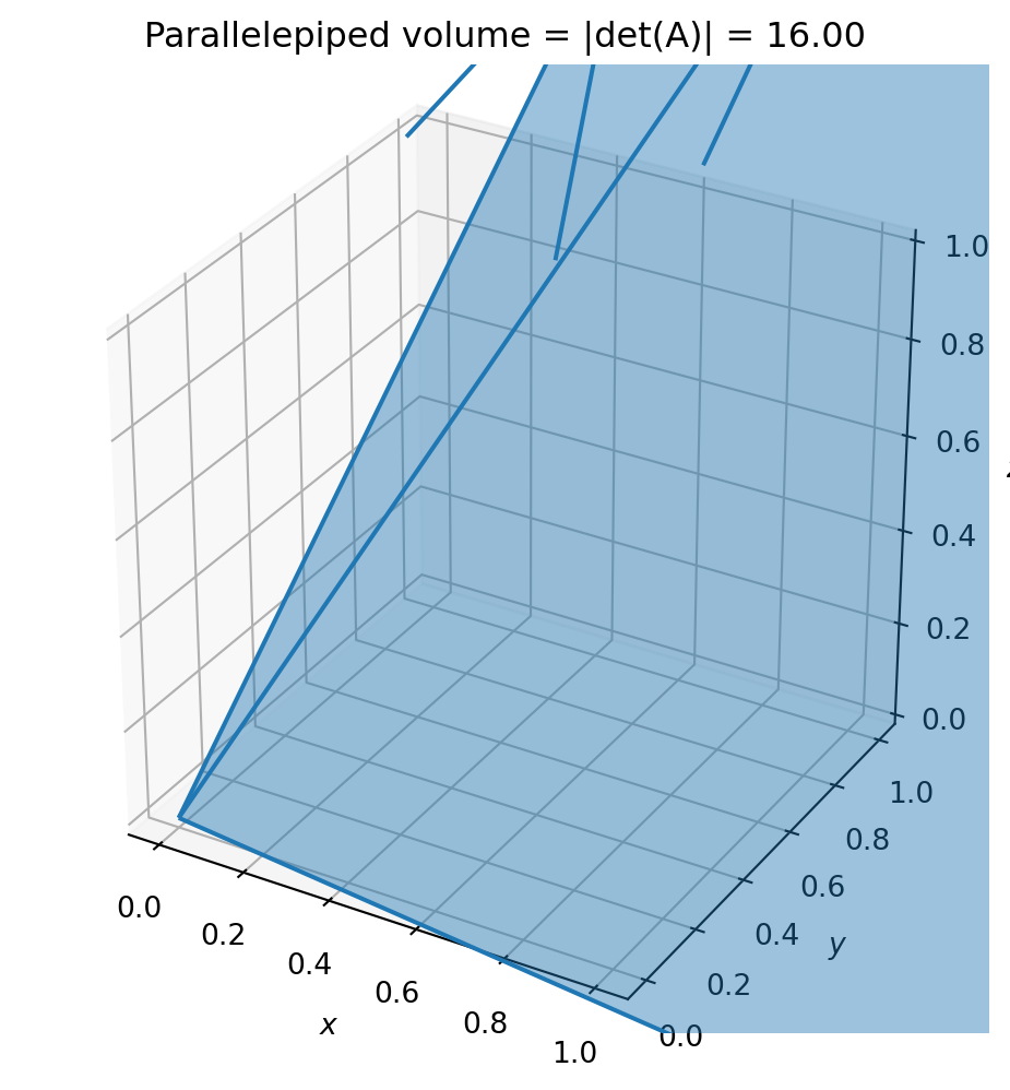
These columns form a parallelepiped.

The volume of this parallelepiped is

\[ |\det(A)|. \]

Volume interpretation

For a \(3\times 3\) matrix \(A\),

\[ |\det(A)| \]

is the volume of the parallelepiped formed by the columns of \(A\).

If \(\det(A)=0\), then the parallelepiped has zero volume. The three columns lie in a plane or line, so they are linearly dependent.

18.13 16.11 Python plot: volume parallelepiped

from mpl_toolkits.mplot3d.art3d import Poly3DCollection

A = np.array([
    [1, 2, 0],
    [0, 1, 3],
    [2, -1, 1]
], dtype=float)

a1, a2, a3 = A[:, 0], A[:, 1], A[:, 2]
detA = np.linalg.det(A)

vertices = np.array([
    [0, 0, 0],
    a1,
    a2,
    a3,
    a1 + a2,
    a1 + a3,
    a2 + a3,
    a1 + a2 + a3
])

faces = [
    [vertices[i] for i in [0, 1, 4, 2]],
    [vertices[i] for i in [0, 1, 5, 3]],
    [vertices[i] for i in [0, 2, 6, 3]],
    [vertices[i] for i in [7, 5, 1, 4]],
    [vertices[i] for i in [7, 6, 2, 4]],
    [vertices[i] for i in [7, 5, 3, 6]]
]

fig = plt.figure(figsize=(7, 6))
ax = fig.add_subplot(111, projection="3d")
poly = Poly3DCollection(faces, alpha=0.25)
ax.add_collection3d(poly)

for v, label in [(a1, "$a_1$"), (a2, "$a_2$"), (a3, "$a_3$")]:
    ax.quiver(0, 0, 0, v[0], v[1], v[2], length=1, normalize=False)
    ax.text(v[0], v[1], v[2], label)

ax.set_xlabel("$x$")
ax.set_ylabel("$y$")
ax.set_zlabel("$z$")
ax.set_title(f"Parallelepiped volume = |det(A)| = {abs(detA):.2f}")
ax.set_box_aspect([1, 1, 1])
plt.show()

18.14 16.12 Determinants and invertibility

The determinant gives a test for invertibility.

Determinant test for invertibility

A square matrix \(A\) is invertible if and only if

\[ \det(A)\ne 0. \]

This connects determinant to the Invertible Matrix Theorem.

For an \(n\times n\) matrix \(A\), the following are equivalent:

\(A\) is invertible,
the columns of \(A\) are linearly independent,
the columns of \(A\) span \(\mathbb{R}^n\),
\(Ax=0\) has only the trivial solution,
\(Ax=b\) has a unique solution for every \(b\),
\(\det(A)\ne 0\).

Geometrically, invertibility means no collapse of volume.

18.15 16.13 Determinant and row operations

Row operations affect determinants in predictable ways.

18.15.1 Row swap

Swapping two rows changes the sign of the determinant.

If \(B\) is obtained from \(A\) by swapping two rows, then

\[ \det(B)=-\det(A). \]

18.15.2 Row scaling

Multiplying one row by a scalar \(c\) multiplies the determinant by \(c\).

If \(B\) is obtained from \(A\) by multiplying one row by \(c\), then

\[ \det(B)=c\det(A). \]

18.15.3 Row replacement

Adding a multiple of one row to another row does not change the determinant.

If \(B\) is obtained from \(A\) by replacing

\[ R_i\leftarrow R_i+cR_j \]

with \(i\ne j\), then

\[ \det(B)=\det(A). \]

Row operation rules for determinants

Row swap changes the sign.
Row scaling by \(c\) multiplies the determinant by \(c\).
Row replacement does not change the determinant.

18.16 16.14 Computing determinants by row reduction

The row-operation rules give a practical determinant algorithm.

Reduce \(A\) to an upper triangular matrix \(U\).

Track row swaps and row scalings.

For an upper triangular matrix

\[ U= \begin{bmatrix} u_{11}&*&\cdots&*\\ 0&u_{22}&\cdots&*\\ \vdots&\vdots&\ddots&\vdots\\ 0&0&\cdots&u_{nn} \end{bmatrix}, \]

the determinant is the product of diagonal entries:

\[ \det(U)=u_{11}u_{22}\cdots u_{nn}. \]

If row reduction used only row replacements and row swaps, then

\[ \det(A)=(-1)^s \det(U), \]

where \(s\) is the number of row swaps.

18.17 16.15 Example: determinant by elimination

Let

\[ A= \begin{bmatrix} 1&2&0\\ 0&1&3\\ 2&-1&1 \end{bmatrix}. \]

Use row replacement:

\[ R_3\leftarrow R_3-2R_1. \]

This gives

\[ \begin{bmatrix} 1&2&0\\ 0&1&3\\ 0&-5&1 \end{bmatrix}. \]

Row replacement does not change determinant.

Now use

\[ R_3\leftarrow R_3+5R_2. \]

This gives

\[ U= \begin{bmatrix} 1&2&0\\ 0&1&3\\ 0&0&16 \end{bmatrix}. \]

Thus

\[ \det(A)=\det(U)=1\cdot 1\cdot 16=16. \]

This agrees with the cofactor expansion.

18.18 16.16 Python: determinant by NumPy

A = np.array([
    [1, 2, 0],
    [0, 1, 3],
    [2, -1, 1]
], dtype=float)

np.linalg.det(A)

16.000000000000007

Because floating-point arithmetic is used, the output may be

\[ 15.999999999999998 \]

instead of exactly \(16\).

For exact symbolic computation, use SymPy.

import sympy as sp

A_sym = sp.Matrix([
    [1, 2, 0],
    [0, 1, 3],
    [2, -1, 1]
])

A_sym.det()

\(\displaystyle 16\)

18.19 16.17 Determinant of triangular matrices

If \(A\) is triangular, then the determinant is the product of diagonal entries.

For an upper triangular matrix

\[ A= \begin{bmatrix} a_{11}&a_{12}&\cdots&a_{1n}\\ 0&a_{22}&\cdots&a_{2n}\\ \vdots&\vdots&\ddots&\vdots\\ 0&0&\cdots&a_{nn} \end{bmatrix}, \]

we have

\[ \det(A)=a_{11}a_{22}\cdots a_{nn}. \]

The same is true for lower triangular matrices.

Triangular determinant

For a triangular matrix \(A\),

\[ \det(A)=\prod_{i=1}^n a_{ii}. \]

18.20 16.18 Determinant of products

Determinants interact beautifully with matrix multiplication.

Multiplicative property

For square matrices \(A\) and \(B\) of the same size,

\[ \det(AB)=\det(A)\det(B). \]

This means volume scaling factors multiply under composition.

If \(B\) scales volume by \(\det(B)\) and \(A\) scales volume by \(\det(A)\), then applying \(B\) first and then \(A\) scales volume by

\[ \det(A)\det(B). \]

18.20.1 Consequences

If \(A\) is invertible, then

\[ \det(A^{-1})=\frac{1}{\det(A)}. \]

Since

\[ AA^{-1}=I, \]

we have

\[ \det(A)\det(A^{-1})=\det(I)=1. \]

Also,

\[ \det(A^k)=\det(A)^k. \]

18.21 16.19 Determinant of a transpose

A matrix and its transpose have the same determinant:

\[ \det(A^T)=\det(A). \]

This means determinants can be studied using rows or columns.

The row and column interpretations are consistent.

18.22 16.20 Scaling one column

The determinant is linear in each column separately.

For example, if one column is multiplied by \(c\), then the determinant is multiplied by \(c\).

Geometrically, stretching one edge of a parallelogram or parallelepiped by \(c\) stretches area or volume by \(c\).

If two columns are equal, the determinant is zero.

If one column is a linear combination of the others, the determinant is zero.

Therefore determinant zero is another way to detect column dependence.

18.23 16.21 Determinant and eigenvalues preview

Later, we will study eigenvalues.

For an \(n\times n\) matrix \(A\), the determinant is related to eigenvalues by

\[ \det(A)=\lambda_1\lambda_2\cdots\lambda_n, \]

counting algebraic multiplicity.

This means the determinant is the product of stretching factors in eigen-directions when such directions are available.

For diagonal matrices, this is already clear.

\[ D= \begin{bmatrix} d_1&0&\cdots&0\\ 0&d_2&\cdots&0\\ \vdots&\vdots&\ddots&\vdots\\ 0&0&\cdots&d_n \end{bmatrix}, \]

then

\[ \det(D)=d_1d_2\cdots d_n. \]

18.24 16.22 Determinants and area under transformations

The determinant tells how a linear transformation changes areas.

If \(A\) is \(2\times 2\) and \(S\) is a region in the plane, then the area of the transformed region \(A(S)\) is

\[ |\det(A)|\cdot \operatorname{area}(S). \]

For example, if

\[ |\det(A)|=3, \]

then every region’s area is scaled by a factor of \(3\).

\[ |\det(A)|=\frac12, \]

then every region’s area is halved.

\[ \det(A)=0, \]

then two-dimensional area collapses to zero.

18.25 16.23 Python plot: transforming a unit square

def plot_unit_square_transform(A, title):
    square = np.array([
        [0, 0],
        [1, 0],
        [1, 1],
        [0, 1]
    ])

    transformed = square @ A.T

    plt.figure(figsize=(6, 6))
    plt.gca().add_patch(Polygon(square, closed=True, alpha=0.25, label="unit square"))
    plt.gca().add_patch(Polygon(transformed, closed=True, alpha=0.35, label="transformed square"))

    plt.arrow(0, 0, A[0, 0], A[1, 0], head_width=0.06, length_includes_head=True)
    plt.arrow(0, 0, A[0, 1], A[1, 1], head_width=0.06, length_includes_head=True)

    plt.axhline(0, linewidth=0.8)
    plt.axvline(0, linewidth=0.8)
    plt.grid(True)
    plt.axis("equal")
    plt.legend()
    plt.title(title + f", det = {np.linalg.det(A):.2f}")
    plt.show()

A = np.array([[2, 1],
              [1, 3]], dtype=float)

plot_unit_square_transform(A, "Unit square transformed by A")

18.26 16.24 Determinants in computation

Determinants are important conceptually, but they are not always the best computational tool.

For example:

To test numerical invertibility, condition number is usually more informative than determinant.
A determinant can be very small or very large simply because dimension is large.
Computing determinant by expansion is inefficient for large matrices.
Row reduction or matrix factorization is the practical method.

In numerical linear algebra, determinant is mainly interpreted through factorizations.

\[ A=LU, \]

then

\[ \det(A)=\det(L)\det(U). \]

If \(L\) has ones on the diagonal, then

\[ \det(L)=1, \]

and

\[ \det(A) \]

is the product of pivots in \(U\), adjusted for row swaps.

18.27 16.25 Algorithmic summary

Algorithm: determinant of a \(2\times 2\) matrix

For

\[ A= \begin{bmatrix} a&b\\ c&d \end{bmatrix}, \]

compute

\[ \det(A)=ad-bc. \]

Algorithm: determinant by row reduction

To compute \(\det(A)\):

Use row operations to reduce \(A\) to an upper triangular matrix \(U\).
Track row swaps.
Avoid row scaling if possible, or track scaling carefully.
Use

\[ \det(U)=\prod_i u_{ii}. \]

Adjust signs and scaling factors from row operations.

Algorithm: area or volume from columns

If \(A\) has columns forming a parallelogram or parallelepiped, then

\[ \text{area or volume}=|\det(A)|. \]

Algorithm: invertibility test

A square matrix \(A\) is invertible if and only if

\[ \det(A)\ne 0. \]

18.28 16.26 Common mistakes

18.28.1 Mistake 1: forgetting the sign

The determinant can be negative.

Area or volume is

\[ |\det(A)|. \]

The sign records orientation.

18.28.2 Mistake 2: confusing determinant with area for nonsquare matrices

The determinant is defined only for square matrices.

Rectangular matrices can change dimension, so ordinary determinant does not apply.

18.28.3 Mistake 3: thinking determinant zero means the matrix is zero

A nonzero matrix can have determinant zero.

For example,

\[ \begin{bmatrix} 1&2\\ 2&4 \end{bmatrix} \]

has determinant zero but is not the zero matrix.

18.28.4 Mistake 4: using cofactor expansion for large matrices

Cofactor expansion is useful for small symbolic examples but inefficient for large matrices.

Use row reduction or factorization.

18.28.5 Mistake 5: treating small determinant as the only sign of numerical difficulty

A small determinant can indicate near collapse, but numerical stability is better measured by condition number and singular values.

18.29 16.27 Chapter summary

For a \(2\times 2\) matrix,

\[ \det \begin{bmatrix} a&b\\ c&d \end{bmatrix} = ad-bc. \]

For a square matrix \(A\), the determinant measures signed volume scaling.

In \(\mathbb{R}^2\),

\[ |\det(A)| \]

is the area of the parallelogram formed by the columns.

In \(\mathbb{R}^3\),

\[ |\det(A)| \]

is the volume of the parallelepiped formed by the columns.

A square matrix is invertible if and only if

\[ \det(A)\ne 0. \]

Row operations affect determinants as follows:

swapping rows changes sign,
scaling a row scales determinant,
adding a multiple of one row to another does not change determinant.

For triangular matrices,

\[ \det(A)=\prod_i a_{ii}. \]

For products,

\[ \det(AB)=\det(A)\det(B). \]

Determinants connect algebra, geometry, orientation, invertibility, and volume.

18.30 Exercises

18.30.1 A. \(2\times 2\) determinants

Compute each determinant and interpret the result geometrically.

\[ \begin{bmatrix} 1&2\\ 3&4 \end{bmatrix} \]

\[ \begin{bmatrix} 2&1\\ 1&3 \end{bmatrix} \]

\[ \begin{bmatrix} 1&2\\ 2&4 \end{bmatrix} \]

\[ \begin{bmatrix} 0&-1\\ 1&0 \end{bmatrix} \]

\[ \begin{bmatrix} 1&0\\ 0&-1 \end{bmatrix} \]

18.30.2 B. Area

For each pair of vectors, compute the area of the parallelogram they form.

\[ a_1= \begin{bmatrix} 2\\ 1 \end{bmatrix}, \qquad a_2= \begin{bmatrix} 1\\ 3 \end{bmatrix}. \]

\[ a_1= \begin{bmatrix} 1\\ 2 \end{bmatrix}, \qquad a_2= \begin{bmatrix} 2\\ 4 \end{bmatrix}. \]

\[ a_1= \begin{bmatrix} 3\\ 0 \end{bmatrix}, \qquad a_2= \begin{bmatrix} 0\\ 5 \end{bmatrix}. \]

18.30.3 C. \(3\times 3\) determinants

Compute each determinant.

\[ \begin{bmatrix} 1&2&0\\ 0&1&3\\ 2&-1&1 \end{bmatrix} \]

\[ \begin{bmatrix} 1&0&0\\ 0&2&0\\ 0&0&3 \end{bmatrix} \]

\[ \begin{bmatrix} 1&2&3\\ 2&4&6\\ 0&1&1 \end{bmatrix} \]

\[ \begin{bmatrix} 0&1&2\\ 1&0&3\\ 4&5&6 \end{bmatrix} \]

18.30.4 D. Volume

Compute the volume of the parallelepiped formed by the columns of each matrix in Exercise C.

18.30.5 E. Row operations

Suppose \(\det(A)=5\) for a \(3\times 3\) matrix.

Find the determinant after each operation.

Swap rows \(1\) and \(2\).
Multiply row \(3\) by \(4\).
Replace row \(2\) by \(R_2-7R_1\).
Multiply the whole matrix by \(2\).
Swap two rows twice.

18.30.6 F. Determinant properties

Let

\[ A= \begin{bmatrix} 1&2\\ 3&4 \end{bmatrix}, \qquad B= \begin{bmatrix} 2&0\\ 1&3 \end{bmatrix}. \]

Compute \(\det(A)\).
Compute \(\det(B)\).
Compute \(\det(AB)\).
Verify that

\[ \det(AB)=\det(A)\det(B). \]

Compute \(\det(A^{-1})\).

18.30.7 G. Python exercises

Use NumPy to compute determinants of several \(2\times 2\) and \(3\times 3\) matrices.
Use SymPy to compute exact determinants.
Plot the parallelogram formed by two vectors and label its area.
Plot a transformed unit square under a \(2\times 2\) matrix.
Experiment with matrices whose columns become nearly dependent and observe how the determinant changes.
Compare determinant with condition number for nearly singular matrices.

18.30.8 H. Reflection

Write a short paragraph answering each question.

Why does determinant zero mean volume collapse?
Why does determinant nonzero imply invertibility?
What does the sign of determinant mean geometrically?
Why does \(\det(AB)=\det(A)\det(B)\) make sense from the viewpoint of volume scaling?
Why is determinant important conceptually but not always the best numerical diagnostic?

18.31 AI-age connection

Determinants measure how linear transformations scale volume. In data science and AI, this idea appears in change of variables, probability densities, normalizing flows, optimization geometry, numerical stability, and invertibility. Although modern computations often use singular values and condition numbers instead of determinants for stability, the determinant remains a powerful conceptual bridge between algebra, geometry, and volume.