Opening question
Linear algebra is not only about solving equations and transforming vectors. It is also about geometry.
To understand geometry, we need ways to measure:
length,
distance,
angle,
perpendicularity,
similarity,
and error.
The central tool is the dot product .
The dot product turns algebraic vectors into geometric objects. It allows us to define orthogonality, projection, least squares, and many algorithms used in computation and data science.
The central question of this chapter is:
How do we measure geometry using vectors?
Learning goals
After studying this chapter, you should be able to:
Compute dot products.
Use the dot product to compute lengths and distances.
Define orthogonality.
Determine whether two vectors are orthogonal.
Compute angles between vectors.
Understand the geometric meaning of dot product.
Use orthogonality to describe subspaces.
Define orthogonal complements.
Understand why orthogonality is important for computation.
Use Python to visualize lengths, distances, angles, and orthogonal vectors.
12.1 The dot product
Let
\[
u=
\begin{bmatrix}
u_1\\
u_2\\
\vdots\\
u_n
\end{bmatrix},
\qquad
v=
\begin{bmatrix}
v_1\\
v_2\\
\vdots\\
v_n
\end{bmatrix}.
\]
The dot product of \(u\) and \(v\) is
\[
u\cdot v=u_1v_1+u_2v_2+\cdots+u_nv_n.
\]
It can also be written as
\[
u^Tv.
\]
For vectors \(u,v\in\mathbb{R}^n\) ,
\[
u\cdot v=u^Tv=\sum_{i=1}^n u_iv_i.
\]
The dot product takes two vectors and produces one number.
12.2 First examples
Let
\[
u=
\begin{bmatrix}
1\\
2\\
3
\end{bmatrix},
\qquad
v=
\begin{bmatrix}
4\\
-1\\
2
\end{bmatrix}.
\]
Then
\[
u\cdot v=1(4)+2(-1)+3(2)=4-2+6=8.
\]
If
\[
a=
\begin{bmatrix}
1\\
2
\end{bmatrix},
\qquad
b=
\begin{bmatrix}
2\\
-1
\end{bmatrix},
\]
then
\[
a\cdot b=1(2)+2(-1)=0.
\]
The value \(0\) will have a special geometric meaning: the vectors are perpendicular.
12.3 Algebraic properties of the dot product
For vectors \(u,v,w\in\mathbb{R}^n\) and scalars \(c\in\mathbb{R}\) :
Symmetry:
\[
u\cdot v=v\cdot u.
\]
Distributivity:
\[
u\cdot(v+w)=u\cdot v+u\cdot w.
\]
Scalar multiplication:
\[
(cu)\cdot v=c(u\cdot v).
\]
Positivity:
\[
u\cdot u\ge 0.
\]
Zero condition:
\[
u\cdot u=0
\]
if and only if
\[
u=0.
\]
These properties make the dot product a useful measurement tool.
12.4 Length of a vector
The length, or norm, of a vector is defined using the dot product.
For
\[
u=
\begin{bmatrix}
u_1\\
u_2\\
\vdots\\
u_n
\end{bmatrix},
\]
the length of \(u\) is
\[
\|u\|=\sqrt{u\cdot u}.
\]
Thus
\[
\|u\|=\sqrt{u_1^2+u_2^2+\cdots+u_n^2}.
\]
The Euclidean norm of \(u\in\mathbb{R}^n\) is
\[
\|u\|=\sqrt{u^Tu}.
\]
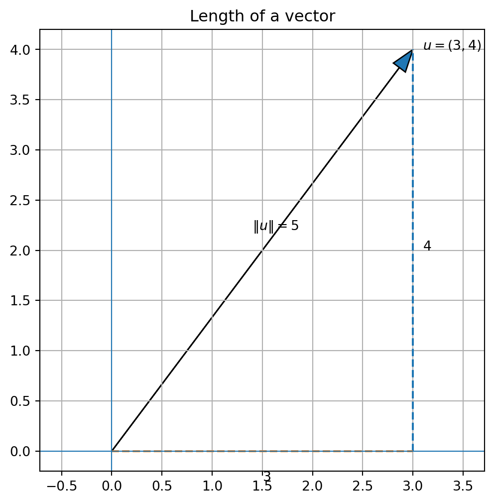
For example,
\[
u=
\begin{bmatrix}
3\\
4
\end{bmatrix}
\]
has length
\[
\|u\|=\sqrt{3^2+4^2}=5.
\]
12.5 Python plot: vector length
import numpy as npimport matplotlib.pyplot as plt= np.array([3 , 4 ], dtype= float )= (6 , 6 ))0 , 0 , u[0 ], u[1 ], head_width= 0.15 , length_includes_head= True )0 ], u[0 ]], [0 , u[1 ]], linestyle= "--" )0 , u[0 ]], [0 , 0 ], linestyle= "--" )0 ] + 0.1 , u[1 ], "$u=(3,4)$" )1.5 , - 0.3 , "$3$" )3.1 , 2 , "$4$" )1.4 , 2.2 , "$ \\ |u \\ |=5$" )0 , linewidth= 0.8 )0 , linewidth= 0.8 )True )"equal" )"Length of a vector" )
12.6 Distance between vectors
The distance between two vectors \(u\) and \(v\) is the length of their difference:
\[
d(u,v)=\|u-v\|.
\]
That is,
\[
d(u,v)=\sqrt{(u-v)\cdot(u-v)}.
\]
In coordinates,
\[
d(u,v)=
\sqrt{(u_1-v_1)^2+\cdots+(u_n-v_n)^2}.
\]
For \(u,v\in\mathbb{R}^n\) ,
\[
d(u,v)=\|u-v\|.
\]
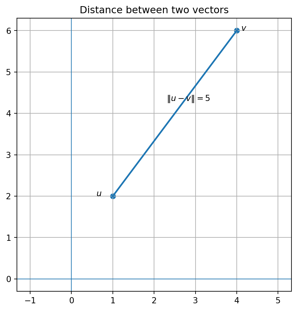
Example
Let
\[
u=
\begin{bmatrix}
1\\
2
\end{bmatrix},
\qquad
v=
\begin{bmatrix}
4\\
6
\end{bmatrix}.
\]
Then
\[
u-v=
\begin{bmatrix}
-3\\
-4
\end{bmatrix}.
\]
So
\[
d(u,v)=\sqrt{(-3)^2+(-4)^2}=5.
\]
12.7 Python plot: distance between points
= np.array([1 , 2 ], dtype= float )= np.array([4 , 6 ], dtype= float )= (6 , 6 ))0 ], v[0 ]], [u[1 ], v[1 ]])0 ], v[0 ]], [u[1 ], v[1 ]], linewidth= 2 )0 ] - 0.4 , u[1 ], "$u$" )0 ] + 0.1 , v[1 ], "$v$" )2.3 , 4.3 , "$ \\ |u-v \\ |=5$" )0 , linewidth= 0.8 )0 , linewidth= 0.8 )True )"equal" )"Distance between two vectors" )
12.8 Unit vectors
A vector with length \(1\) is called a unit vector .
A vector \(u\) is a unit vector if
\[
\|u\|=1.
\]
If \(v\ne 0\) , then we can create a unit vector in the same direction by dividing by its length:
\[
\hat v=\frac{v}{\|v\|}.
\]
This process is called normalization .
Example
Let
\[
v=
\begin{bmatrix}
3\\
4
\end{bmatrix}.
\]
Then
\[
\|v\|=5.
\]
So
\[
\hat v=
\frac{1}{5}
\begin{bmatrix}
3\\
4
\end{bmatrix}
=
\begin{bmatrix}
3/5\\
4/5
\end{bmatrix}.
\]
Check:
\[
\|\hat v\|=
\sqrt{(3/5)^2+(4/5)^2}=1.
\]
12.9 Orthogonality
Two vectors are orthogonal if their dot product is zero.
Vectors \(u,v\in\mathbb{R}^n\) are orthogonal if
\[
u\cdot v=0.
\]
In \(\mathbb{R}^2\) and \(\mathbb{R}^3\) , orthogonal means perpendicular.
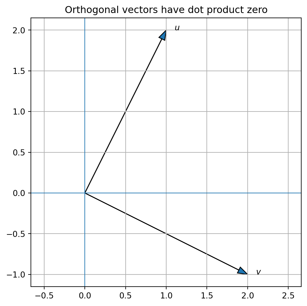
Example
Let
\[
u=
\begin{bmatrix}
1\\
2
\end{bmatrix},
\qquad
v=
\begin{bmatrix}
2\\
-1
\end{bmatrix}.
\]
Then
\[
u\cdot v=1(2)+2(-1)=0.
\]
Therefore \(u\) and \(v\) are orthogonal.
12.10 Python plot: orthogonal vectors
= np.array([1 , 2 ], dtype= float )= np.array([2 , - 1 ], dtype= float )= (6 , 6 ))0 , 0 , u[0 ], u[1 ], head_width= 0.08 , length_includes_head= True )0 , 0 , v[0 ], v[1 ], head_width= 0.08 , length_includes_head= True )0 ] + 0.1 , u[1 ], "$u$" )0 ] + 0.1 , v[1 ], "$v$" )0 , linewidth= 0.8 )0 , linewidth= 0.8 )True )"equal" )"Orthogonal vectors have dot product zero" )print ("u dot v =" , np.dot(u, v))
12.11 Angle between vectors
The dot product is related to angle by the formula
\[
u\cdot v=\|u\|\|v\|\cos\theta,
\]
where \(\theta\) is the angle between \(u\) and \(v\) .
If \(u\) and \(v\) are nonzero, then
\[
\cos\theta=
\frac{u\cdot v}{\|u\|\|v\|}.
\]
Thus
\[
\theta=\cos^{-1}\left(\frac{u\cdot v}{\|u\|\|v\|}\right).
\]
For nonzero vectors \(u,v\in\mathbb{R}^n\) ,
\[
\cos\theta=
\frac{u\cdot v}{\|u\|\|v\|}.
\]
If \(u\cdot v=0\) , then
\[
\cos\theta=0,
\]
so
\[
\theta=\frac{\pi}{2}.
\]
That is why dot product zero means perpendicular.
12.12 Example: computing an angle
Let
\[
u=
\begin{bmatrix}
1\\
1
\end{bmatrix},
\qquad
v=
\begin{bmatrix}
1\\
0
\end{bmatrix}.
\]
Then
\[
u\cdot v=1.
\]
Also,
\[
\|u\|=\sqrt{2},
\qquad
\|v\|=1.
\]
So
\[
\cos\theta=
\frac{1}{\sqrt{2}}.
\]
Therefore
\[
\theta=\frac{\pi}{4}.
\]
The angle is \(45^\circ\) .
12.13 Python: angle between vectors
= np.array([1 , 1 ], dtype= float )= np.array([1 , 0 ], dtype= float )= np.dot(u, v) / (np.linalg.norm(u) * np.linalg.norm(v))= np.arccos(cos_theta)* 180 / np.pi
(0.7853981633974484, 45.00000000000001)
12.14 Cauchy–Schwarz inequality
The angle formula requires
\[
-1\le
\frac{u\cdot v}{\|u\|\|v\|}
\le 1.
\]
Equivalently,
\[
|u\cdot v|\le \|u\|\|v\|.
\]
This is the Cauchy–Schwarz inequality .
For all \(u,v\in\mathbb{R}^n\) ,
\[
|u\cdot v|\le \|u\|\|v\|.
\]
Equality occurs when one vector is a scalar multiple of the other.
This inequality is one of the central inequalities in linear algebra, statistics, optimization, and machine learning.
12.15 Triangle inequality
The distance idea depends on the triangle inequality:
\[
\|u+v\|\le \|u\|+\|v\|.
\]
For all \(u,v\in\mathbb{R}^n\) ,
\[
\|u+v\|\le \|u\|+\|v\|.
\]
Geometrically, the direct path from the origin to \(u+v\) is no longer than the path that first goes to \(u\) and then follows \(v\) .
12.16 Orthogonal sets
A set of vectors \(\{v_1,\ldots,v_k\}\) is an orthogonal set if every pair of distinct vectors is orthogonal:
\[
v_i\cdot v_j=0
\]
whenever \(i\ne j\) .
If each vector also has length \(1\) , the set is orthonormal .
A set \(\{v_1,\ldots,v_k\}\) is orthogonal if
\[
v_i\cdot v_j=0\quad \text{for } i\ne j.
\]
It is orthonormal if it is orthogonal and
\[
\|v_i\|=1
\]
for every \(i\) .
Example
The standard basis vectors
\[
e_1,e_2,\ldots,e_n
\]
form an orthonormal set.
12.17 Orthogonal nonzero vectors are independent
Any set of nonzero mutually orthogonal vectors is linearly independent.
Why?
Suppose
\[
c_1v_1+\cdots+c_kv_k=0.
\]
Take the dot product with \(v_j\) :
\[
(c_1v_1+\cdots+c_kv_k)\cdot v_j=0\cdot v_j.
\]
Because the vectors are orthogonal, all terms vanish except one:
\[
c_j(v_j\cdot v_j)=0.
\]
Since \(v_j\ne 0\) ,
\[
v_j\cdot v_j=\|v_j\|^2\ne 0.
\]
Therefore
\[
c_j=0.
\]
This works for every \(j\) , so all coefficients are zero.
Thus the vectors are linearly independent.
12.18 Orthogonal complement
Let \(W\) be a subspace of \(\mathbb{R}^n\) .
The orthogonal complement of \(W\) is the set of all vectors orthogonal to every vector in \(W\) .
For a subspace \(W\subseteq\mathbb{R}^n\) ,
\[
W^\perp=
\{x\in\mathbb{R}^n:x\cdot w=0\text{ for every }w\in W\}.
\]
The orthogonal complement \(W^\perp\) is also a subspace.
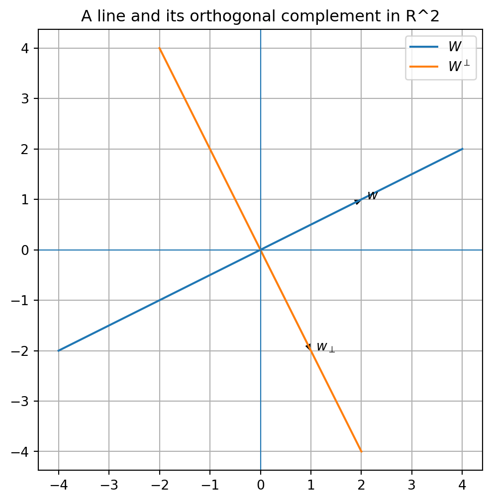
12.19 Example: orthogonal complement of a line
Let
\[
W=\operatorname{span}
\left\{
\begin{bmatrix}
2\\
1
\end{bmatrix}
\right\}
\subseteq \mathbb{R}^2.
\]
A vector
\[
x=
\begin{bmatrix}
a\\
b
\end{bmatrix}
\]
is in \(W^\perp\) if
\[
x\cdot
\begin{bmatrix}
2\\
1
\end{bmatrix}
=0.
\]
That is,
\[
2a+b=0.
\]
So
\[
b=-2a.
\]
Thus
\[
x=
\begin{bmatrix}
a\\
-2a
\end{bmatrix}
=
a
\begin{bmatrix}
1\\
-2
\end{bmatrix}.
\]
Therefore
\[
W^\perp=
\operatorname{span}
\left\{
\begin{bmatrix}
1\\
-2
\end{bmatrix}
\right\}.
\]
12.20 Python plot: a subspace and its orthogonal complement
= np.array([2 , 1 ], dtype= float )= np.array([1 , - 2 ], dtype= float )= np.linspace(- 2 , 2 , 100 )= np.outer(t, w)= np.outer(t, wp)= (6 , 6 ))0 ], line_W[:, 1 ], label= "$W$" )0 ], line_Wp[:, 1 ], label= "$W^ \\ perp$" )0 , 0 , w[0 ], w[1 ], head_width= 0.08 , length_includes_head= True )0 , 0 , wp[0 ], wp[1 ], head_width= 0.08 , length_includes_head= True )0 ] + 0.1 , w[1 ], "$w$" )0 ] + 0.1 , wp[1 ], "$w_ \\ perp$" )0 , linewidth= 0.8 )0 , linewidth= 0.8 )True )"equal" )"A line and its orthogonal complement in R^2" )
12.21 Orthogonal complements and matrices
The nullspace of a matrix is connected to orthogonality.
Let
\[
A=
\begin{bmatrix}
--- a_1^T ---\\
--- a_2^T ---\\
\vdots\\
--- a_m^T ---
\end{bmatrix}
\]
where the rows are \(a_1^T,\ldots,a_m^T\) .
The equation
\[
Ax=0
\]
means
\[
a_1\cdot x=0,
\]
\[
a_2\cdot x=0,
\]
and so on.
Thus \(x\) is orthogonal to every row of \(A\) .
Therefore
\[
\operatorname{Null}(A)=\operatorname{Row}(A)^\perp.
\]
For any matrix \(A\) ,
\[
\operatorname{Null}(A)=\operatorname{Row}(A)^\perp.
\]
This is one of the first appearances of the fundamental theorem of linear algebra.
12.22 Why orthogonality matters computationally
Orthogonality is powerful because it simplifies calculations.
If \(v_1,\ldots,v_k\) are orthogonal, then dot products between different basis directions vanish.
This makes many formulas simple.
For example, if \(\{q_1,\ldots,q_k\}\) is orthonormal and
\[
x=c_1q_1+\cdots+c_kq_k,
\]
then
\[
c_j=x\cdot q_j.
\]
Why?
Take the dot product with \(q_j\) :
\[
x\cdot q_j
=
(c_1q_1+\cdots+c_kq_k)\cdot q_j
=
c_j(q_j\cdot q_j)
=
c_j.
\]
This is the foundation of orthogonal projection, Fourier series, QR factorization, PCA, and the SVD.
12.23 Python: orthogonal coordinates
= np.array([1 , 0 ], dtype= float )= np.array([0 , 1 ], dtype= float )= np.array([3 , 4 ], dtype= float )= np.dot(x, q1)= np.dot(x, q2)
For a rotated orthonormal basis:
= np.array([1 , 1 ], dtype= float ) / np.sqrt(2 )= np.array([1 , - 1 ], dtype= float ) / np.sqrt(2 )= np.array([3 , 1 ], dtype= float )= np.dot(x, q1)= np.dot(x, q2)= np.array([c1, c2])
array([2.82842712, 1.41421356])
Reconstruct the vector:
The dot products give the coordinates because the basis is orthonormal.
12.24 Algorithmic summary
For \(u\in\mathbb{R}^n\) ,
\[
\|u\|=\sqrt{u\cdot u}.
\]
For \(u,v\in\mathbb{R}^n\) ,
\[
d(u,v)=\|u-v\|.
\]
Vectors \(u\) and \(v\) are orthogonal if
\[
u\cdot v=0.
\]
For nonzero vectors \(u\) and \(v\) ,
\[
\theta=
\cos^{-1}
\left(
\frac{u\cdot v}{\|u\|\|v\|}
\right).
\]
To find \(W^\perp\) when \(W=\operatorname{span}\{w_1,\ldots,w_k\}\) :
Let \(x\) be an unknown vector.
Solve the system
\[
x\cdot w_1=0,\quad \ldots,\quad x\cdot w_k=0.
\]
Write the solution as a span.
12.25 Common mistakes
Mistake 1: confusing dot product with matrix multiplication
The dot product of two vectors produces a scalar.
Matrix-vector multiplication produces a vector.
Mistake 3: forgetting to normalize
Orthogonal vectors are perpendicular.
Orthonormal vectors are perpendicular and have length \(1\) .
Mistake 5: thinking \(W^\perp\) contains vectors outside the ambient space
If \(W\subseteq\mathbb{R}^n\) , then \(W^\perp\subseteq\mathbb{R}^n\) .
12.26 Chapter summary
The dot product is
\[
u\cdot v=u^Tv=\sum_{i=1}^n u_iv_i.
\]
The length of a vector is
\[
\|u\|=\sqrt{u\cdot u}.
\]
The distance between two vectors is
\[
d(u,v)=\|u-v\|.
\]
Two vectors are orthogonal if
\[
u\cdot v=0.
\]
For nonzero vectors,
\[
\cos\theta=
\frac{u\cdot v}{\|u\|\|v\|}.
\]
The Cauchy–Schwarz inequality says
\[
|u\cdot v|\le \|u\|\|v\|.
\]
The orthogonal complement of a subspace \(W\) is
\[
W^\perp=\{x:x\cdot w=0\text{ for all }w\in W\}.
\]
For a matrix \(A\) ,
\[
\operatorname{Null}(A)=\operatorname{Row}(A)^\perp.
\]
Orthogonality simplifies computation and prepares the way for projections, least squares, QR factorization, PCA, and the SVD.
Exercises
A. Dot products
Compute each dot product.
\[
\begin{bmatrix}1\\2\\3\end{bmatrix}
\cdot
\begin{bmatrix}4\\-1\\2\end{bmatrix}
\]
\[
\begin{bmatrix}1\\2\end{bmatrix}
\cdot
\begin{bmatrix}2\\-1\end{bmatrix}
\]
\[
\begin{bmatrix}3\\4\end{bmatrix}
\cdot
\begin{bmatrix}3\\4\end{bmatrix}
\]
\[
\begin{bmatrix}1\\-1\\2\\0\end{bmatrix}
\cdot
\begin{bmatrix}2\\3\\1\\5\end{bmatrix}
\]
B. Length and distance
Find the length of
\[
\begin{bmatrix}3\\4\end{bmatrix}.
\]
Find the length of
\[
\begin{bmatrix}1\\2\\2\end{bmatrix}.
\]
Find the distance between
\[
u=\begin{bmatrix}1\\2\end{bmatrix}
\]
and
\[
v=\begin{bmatrix}4\\6\end{bmatrix}.
\]
Normalize
\[
v=\begin{bmatrix}3\\4\end{bmatrix}.
\]
C. Orthogonality
Determine whether each pair is orthogonal.
\[
\begin{bmatrix}1\\2\end{bmatrix},
\begin{bmatrix}2\\-1\end{bmatrix}
\]
\[
\begin{bmatrix}1\\1\\1\end{bmatrix},
\begin{bmatrix}1\\-1\\0\end{bmatrix}
\]
\[
\begin{bmatrix}1\\0\\1\end{bmatrix},
\begin{bmatrix}1\\1\\-1\end{bmatrix}
\]
\[
\begin{bmatrix}2\\-1\\3\end{bmatrix},
\begin{bmatrix}1\\2\\0\end{bmatrix}
\]
D. Angles
Compute the angle between each pair of vectors.
\[
\begin{bmatrix}1\\0\end{bmatrix},
\begin{bmatrix}1\\1\end{bmatrix}
\]
\[
\begin{bmatrix}1\\0\end{bmatrix},
\begin{bmatrix}0\\1\end{bmatrix}
\]
\[
\begin{bmatrix}1\\2\end{bmatrix},
\begin{bmatrix}2\\1\end{bmatrix}
\]
E. Orthogonal complements
Find a basis for \(W^\perp\) .
\[
W=\operatorname{span}
\left\{
\begin{bmatrix}2\\1\end{bmatrix}
\right\}
\subseteq\mathbb{R}^2.
\]
\[
W=\operatorname{span}
\left\{
\begin{bmatrix}1\\0\\1\end{bmatrix}
\right\}
\subseteq\mathbb{R}^3.
\]
\[
W=\operatorname{span}
\left\{
\begin{bmatrix}1\\0\\1\end{bmatrix},
\begin{bmatrix}0\\1\\1\end{bmatrix}
\right\}
\subseteq\mathbb{R}^3.
\]
F. Nullspace and row space
For each matrix, find \(\operatorname{Null}(A)\) and verify that it is orthogonal to the row space.
\[
A=
\begin{bmatrix}
1&2
\end{bmatrix}
\]
\[
A=
\begin{bmatrix}
1&0&1\\
0&1&1
\end{bmatrix}
\]
\[
A=
\begin{bmatrix}
1&2&3\\
2&4&6
\end{bmatrix}
\]
G. Python exercises
Use NumPy to compute dot products, norms, and distances.
Plot two orthogonal vectors in \(\mathbb{R}^2\) .
Write a Python function that computes the angle between two nonzero vectors.
Plot a line and its orthogonal complement in \(\mathbb{R}^2\) .
Use SymPy to find the nullspace of a matrix and check orthogonality with the rows.
H. Reflection
Write a short paragraph answering each question.
Why does the dot product measure geometric alignment?
Why does dot product zero mean perpendicular?
Why are orthogonal vectors easier to use as building blocks?
How does the nullspace relate to orthogonality?
Why is orthogonality important for computation and AI?
AI-age connection
Orthogonality is one of the most important ideas in computational linear algebra. It makes coordinates stable, separates information into independent directions, and turns difficult fitting problems into geometric projection problems. Orthogonal bases appear in QR factorization, Fourier analysis, PCA, the SVD, and modern data compression. In high-dimensional data, dot products and angles are used to measure similarity, compare embeddings, and understand model geometry.