Opening question
Eigenvalues and eigenvectors reveal the special directions of a square matrix.
But many important matrices are not square.
A data matrix may have thousands of rows and hundreds of columns. An image matrix may be rectangular. A design matrix in least squares is often tall. A transformation may map one dimension into another.
So we need a factorization that works for every matrix .
The singular value decomposition, or SVD , does exactly that.
For any real \(m\times n\) matrix \(A\) , the SVD writes
\[
A=U\Sigma V^T,
\]
where:
\(U\) has orthonormal columns,\(V\) has orthonormal columns,\(\Sigma\) is diagonal-shaped with nonnegative entries.
The SVD says that every matrix transformation can be understood as three steps:
\[
\text{rotate/reflect} \quad \longrightarrow \quad \text{stretch/compress} \quad \longrightarrow \quad \text{rotate/reflect}.
\]
The central question of this chapter is:
What are the natural input and output directions of any matrix?
The answer is singular vectors and singular values.
Learning goals
After studying this chapter, you should be able to:
Define singular values and singular vectors.
Explain the singular value decomposition \(A=U\Sigma V^T\) .
Connect the SVD to eigenvalues of \(A^TA\) and \(AA^T\) .
Interpret singular values as stretching factors.
Understand the four fundamental subspaces through the SVD.
Compute the SVD using Python.
Use the SVD to find rank and numerical rank.
Construct low-rank approximations.
Apply the SVD to image compression.
Connect the SVD to PCA, least squares, data science, and AI.
21.1 Why eigenvalues are not enough
Eigenvalues require a square matrix.
If
\[
A
\]
is \(m\times n\) with \(m\ne n\) , then the equation
\[
Av=\lambda v
\]
does not make sense because \(Av\in\mathbb{R}^m\) while \(v\in\mathbb{R}^n\) .
Even when \(A\) is square, eigenvectors may not form an orthonormal basis, and eigenvalues may be complex.
The SVD avoids these problems.
It works for every real matrix:
square or rectangular,
invertible or singular,
full rank or rank deficient,
diagonalizable or not.
21.2 The geometric picture
A matrix
\[
A:\mathbb{R}^n\to\mathbb{R}^m
\]
takes input vectors in \(\mathbb{R}^n\) and produces output vectors in \(\mathbb{R}^m\) .
The SVD finds special orthonormal input directions
\[
v_1,\ldots,v_n
\]
and special orthonormal output directions
\[
u_1,\ldots,u_m
\]
such that
\[
Av_i=\sigma_i u_i
\]
for singular values
\[
\sigma_i\ge 0.
\]
This means:
\(v_i\) is a special input direction,\(u_i\) is the corresponding output direction,\(\sigma_i\) is the stretching factor.
So the SVD is like the eigenvector equation, but it allows input and output directions to live in different spaces.
For the SVD,
\[
Av_i=\sigma_i u_i.
\]
21.3 The singular value decomposition
For every real \(m\times n\) matrix \(A\) , there exist orthogonal matrices \(U\) and \(V\) and a diagonal-shaped matrix \(\Sigma\) such that
\[
A=U\Sigma V^T.
\]
Here:
\(U\) is an \(m\times m\) orthogonal matrix,\(V\) is an \(n\times n\) orthogonal matrix,\(\Sigma\) is an \(m\times n\) diagonal-shaped matrix,the diagonal entries of \(\Sigma\) are nonnegative singular values.
The singular values are usually ordered:
\[
\sigma_1\ge \sigma_2\ge \cdots \ge \sigma_r>0,
\]
where
\[
r=\operatorname{rank}(A).
\]
The remaining singular values are zero.
21.4 Reduced SVD
In computation, the reduced SVD is often more convenient.
If \(A\) has rank \(r\) , then
\[
A=U_r\Sigma_rV_r^T,
\]
where:
\(U_r\) is \(m\times r\) with orthonormal columns,\(\Sigma_r\) is \(r\times r\) diagonal with positive singular values,\(V_r\) is \(n\times r\) with orthonormal columns.
The reduced SVD only keeps the nonzero singular directions.
If \(\operatorname{rank}(A)=r\) , then
\[
A=U_r\Sigma_rV_r^T.
\]
This form is compact and reveals the essential structure of \(A\) .
21.5 How the SVD acts on a vector
Suppose
\[
A=U\Sigma V^T.
\]
Then
\[
Ax=U\Sigma V^Tx.
\]
This means the transformation happens in three steps:
\(V^Tx\) : express \(x\) in the right singular vector coordinates,\(\Sigma V^Tx\) : stretch or shrink each coordinate by a singular value,\(U\Sigma V^Tx\) : rotate or reflect into the output space.
So the SVD decomposes any linear transformation into:
\[
\text{orthogonal change of input coordinates}
\quad \to \quad
\text{axis scaling}
\quad \to \quad
\text{orthogonal change of output coordinates}.
\]
This is the most geometric matrix factorization.
21.6 Singular values from \(A^TA\)
The matrix
\[
A^TA
\]
is always symmetric and positive semidefinite.
Therefore it has an orthonormal eigenbasis and nonnegative eigenvalues.
The singular values of \(A\) are square roots of the eigenvalues of \(A^TA\) .
If
\[
A^TAv_i=\lambda_i v_i,
\]
with \(\lambda_i\ge 0\) , then
\[
\sigma_i=\sqrt{\lambda_i}
\]
is a singular value of \(A\) .
The vectors \(v_i\) are the right singular vectors .
Once \(v_i\) is known and \(\sigma_i>0\) , the corresponding left singular vector is
\[
u_i=\frac{Av_i}{\sigma_i}.
\]
21.7 Why \(A^TA\) is positive semidefinite
For any vector \(x\) ,
\[
x^T(A^TA)x=(Ax)^T(Ax)=\|Ax\|^2\ge 0.
\]
Thus \(A^TA\) is positive semidefinite.
This is why its eigenvalues are nonnegative, and why singular values are real and nonnegative.
The SVD is built from the spectral theorem applied to \(A^TA\) .
21.8 A simple diagonal example
Let
\[
A=
\begin{bmatrix}
3&0\\
0&1
\end{bmatrix}.
\]
Then
\[
A^TA=
\begin{bmatrix}
9&0\\
0&1
\end{bmatrix}.
\]
The eigenvalues of \(A^TA\) are \(9\) and \(1\) .
Therefore the singular values are
\[
\sigma_1=3,
\qquad
\sigma_2=1.
\]
The right singular vectors are
\[
e_1,\ e_2.
\]
The left singular vectors are also
\[
e_1,\ e_2.
\]
So
\[
A=U\Sigma V^T
\]
with
\[
U=I,\quad
\Sigma=
\begin{bmatrix}
3&0\\
0&1
\end{bmatrix},
\quad
V=I.
\]
21.9 Example with reflection
Let
\[
A=
\begin{bmatrix}
0&2\\
3&0
\end{bmatrix}.
\]
Compute
\[
A^TA=
\begin{bmatrix}
0&3\\
2&0
\end{bmatrix}
\begin{bmatrix}
0&2\\
3&0
\end{bmatrix}
=
\begin{bmatrix}
9&0\\
0&4
\end{bmatrix}.
\]
The eigenvalues are \(9\) and \(4\) , so the singular values are
\[
3
\quad \text{and} \quad
2.
\]
This matrix swaps directions and scales them. The SVD separates these actions into orthogonal directions and nonnegative stretches.
21.10 Python: computing the SVD
import numpy as npimport matplotlib.pyplot as plt= np.array([[0 , 2 ],3 , 0 ]], dtype= float )= np.linalg.svd(A)
(array([[ 0., -1.],
        [-1.,  0.]]),
 array([3., 2.]),
 array([[-1., -0.],
        [-0., -1.]]))
The vector s stores the singular values.
To reconstruct the matrix:
= np.zeros_like(A)= U @ Sigma @ Vt
array([[0., 2.],
       [3., 0.]])
Check reconstruction error:
- A_reconstructed)
21.11 Singular values as stretching factors
The largest singular value has an important geometric meaning:
\[
\sigma_1=\max_{\|x\|=1}\|Ax\|.
\]
That is, \(\sigma_1\) is the largest amount that \(A\) stretches any unit vector.
The smallest singular value, when \(A\) is square and full rank, is
\[
\sigma_n=\min_{\|x\|=1}\|Ax\|.
\]
So singular values describe how the unit sphere is transformed.
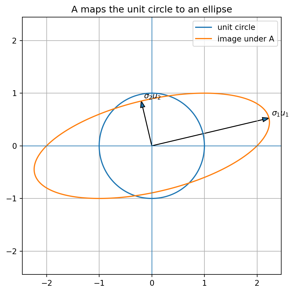
A matrix maps the unit circle in \(\mathbb{R}^2\) to an ellipse in \(\mathbb{R}^2\) .
The semiaxis lengths of that ellipse are the singular values.
21.12 Python plot: unit circle to ellipse
def plot_circle_to_ellipse(A, title):= np.linspace(0 , 2 * np.pi, 400 )= np.vstack([np.cos(theta), np.sin(theta)])= A @ circle= np.linalg.svd(A)= (6 , 6 ))0 ], circle[1 ], label= "unit circle" )0 ], ellipse[1 ], label= "image under A" )for i in range (2 ):= U[:, i]0 , 0 , s[i]* ui[0 ], s[i]* ui[1 ],= 0.08 , length_includes_head= True )* ui[0 ] + 0.05 , s[i]* ui[1 ] + 0.05 , f"$ \\ sigma_ { i+ 1 } u_ { i+ 1 } $" )0 , linewidth= 0.8 )0 , linewidth= 0.8 )True )"equal" )= np.array([[2 , 1 ],0 , 1 ]], dtype= float )"A maps the unit circle to an ellipse" )
The singular values are the semiaxis lengths of the ellipse.
The left singular vectors give the directions of the ellipse axes.
21.14 Left singular vectors and output directions
The left singular vectors \(u_i\) are directions in the output space.
For positive singular values,
\[
u_i=\frac{Av_i}{\sigma_i}.
\]
They also satisfy
\[
AA^Tu_i=\sigma_i^2u_i.
\]
Thus left singular vectors are eigenvectors of
\[
AA^T.
\]
The nonzero eigenvalues of \(A^TA\) and \(AA^T\) are the same.
21.15 Python: checking singular vector relations
= np.array([[2 , 1 ],0 , 1 ]], dtype= float )= np.linalg.svd(A)= Vt.Tfor i in range (len (s)):print ("i =" , i)print ("sigma =" , s[i])print ("A v_i =" , A @ V[:, i])print ("sigma_i u_i =" , s[i] * U[:, i])print ()
i = 0
sigma = 2.2882456112707374
A v_i = [2.22703273 0.52573111]
sigma_i u_i = [2.22703273 0.52573111]

i = 1
sigma = 0.8740320488976421
A v_i = [-0.20081142  0.85065081]
sigma_i u_i = [-0.20081142  0.85065081]
Also check eigenvalue relations:
(array([[4., 2.],
        [2., 2.]]),
 array([[ 0.85065081, -0.52573111],
        [ 0.52573111,  0.85065081]]),
 array([5.23606798, 0.76393202]))
for i in range (len (s)):print ("A^T A v_i =" , A.T @ A @ V[:, i])print ("sigma_i^2 v_i =" , (s[i]** 2 ) * V[:, i])print ()
A^T A v_i = [4.45406546 2.75276384]
sigma_i^2 v_i = [4.45406546 2.75276384]

A^T A v_i = [-0.40162283  0.64983939]
sigma_i^2 v_i = [-0.40162283  0.64983939]
21.16 Rank and singular values
The rank of a matrix is the number of nonzero singular values.
For any matrix \(A\) ,
\[
\operatorname{rank}(A)=\#\{i:\sigma_i>0\}.
\]
In exact mathematics, singular values are either zero or positive.
In numerical computation, very small singular values indicate directions that are nearly collapsed.
This leads to the idea of numerical rank .
21.17 Numerical rank
In floating-point computation, a singular value may not be exactly zero.
Instead, we use a tolerance.
For example, if
\[
\sigma_i < 10^{-10},
\]
we might treat it as zero.
Numerical rank is the number of singular values that are large relative to a chosen tolerance.
= np.array([1 , 2 ],2 , 4 ],3 , 6 ]= float )= np.linalg.svd(A, compute_uv= False )
array([8.36660027e+00, 4.11373409e-16])
This matrix has dependent columns, so one singular value should be zero up to numerical roundoff.
21.18 Condition number
For an invertible square matrix \(A\) , the condition number in the Euclidean norm is
\[
\kappa(A)=\frac{\sigma_{\max}}{\sigma_{\min}}.
\]
A large condition number means that the matrix stretches some directions much more than others.
This can make solving linear systems sensitive to small changes in data.
For an invertible square matrix,
\[
\kappa(A)=\frac{\sigma_1}{\sigma_n}.
\]
If \(\sigma_n\) is close to zero, the matrix is close to singular.
21.19 Python: condition number
= np.array([[2 , 0 ],0 , 1 ]], dtype= float )= np.array([[1 , 0 ],0 , 0.001 ]], dtype= float )
The second matrix is ill-conditioned because it nearly collapses one direction.
21.20 The four fundamental subspaces through SVD
Suppose
\[
A=U\Sigma V^T
\]
has rank \(r\) .
Let
\[
v_1,\ldots,v_n
\]
be the right singular vectors and
\[
u_1,\ldots,u_m
\]
be the left singular vectors.
Then:
\[
\operatorname{Row}(A)=\operatorname{span}\{v_1,\ldots,v_r\},
\]
\[
\operatorname{Null}(A)=\operatorname{span}\{v_{r+1},\ldots,v_n\},
\]
\[
\operatorname{Col}(A)=\operatorname{span}\{u_1,\ldots,u_r\},
\]
and
\[
\operatorname{Null}(A^T)=\operatorname{span}\{u_{r+1},\ldots,u_m\}.
\]
The SVD gives orthonormal bases for all four fundamental subspaces.
This is one of the most complete structural descriptions of a matrix.
21.22 Python: outer product reconstruction
= np.array([[2 , 1 ],0 , 1 ],1 , 0 ]], dtype= float )= np.linalg.svd(A, full_matrices= False )= np.zeros_like(A)for i in range (len (s)):+= s[i] * np.outer(U[:, i], Vt[i, :])
(array([[2., 1.],
        [0., 1.],
        [1., 0.]]),
 array([[ 2.00000000e+00,  1.00000000e+00],
        [-1.11022302e-16,  1.00000000e+00],
        [ 1.00000000e+00, -1.66533454e-16]]))
21.23 Low-rank approximation
The outer product form suggests approximating \(A\) by keeping only the largest singular values.
Define
\[
A_k=\sum_{i=1}^k \sigma_i u_iv_i^T.
\]
Then \(A_k\) has rank at most \(k\) .
The larger singular values often contain the most important structure of the matrix.
The smaller singular values often represent fine detail or noise.
The rank-\(k\) truncated SVD is
\[
A_k=\sum_{i=1}^k \sigma_i u_iv_i^T.
\]
The Eckart–Young theorem says that \(A_k\) is the best rank-\(k\) approximation to \(A\) in the Euclidean matrix norm and Frobenius norm.
21.24 Best low-rank approximation
Among all matrices \(B\) with rank at most \(k\) , the truncated SVD
\[
A_k=\sum_{i=1}^k \sigma_i u_iv_i^T
\]
minimizes
\[
\|A-B\|.
\]
This theorem is one of the reasons the SVD is so important in data science.
It gives the best way to compress a matrix using a fixed number of dimensions.
21.25 Python: low-rank approximation
= np.random.default_rng(0 )# Create a simple low-rank-ish data matrix = 60 , 40 = np.linspace(0 , 1 , m)= np.linspace(0 , 1 , n)= (2 * np.pi* t), np.cos(2 * np.pi* x))+ 0.5 * np.outer(np.cos(4 * np.pi* t), np.sin(np.pi* x))# Add small noise = A + 0.1 * rng.normal(size= (m, n))= np.linalg.svd(A_noisy, full_matrices= False )def truncated_svd(U, s, Vt, k):return (U[:, :k] * s[:k]) @ Vt[:k, :]= truncated_svd(U, s, Vt, 1 )= truncated_svd(U, s, Vt, 2 )= truncated_svd(U, s, Vt, 5 )- A1), np.linalg.norm(A_noisy - A2), np.linalg.norm(A_noisy - A5)
(11.945793990535545, 4.720868298144663, 4.149151018731544)
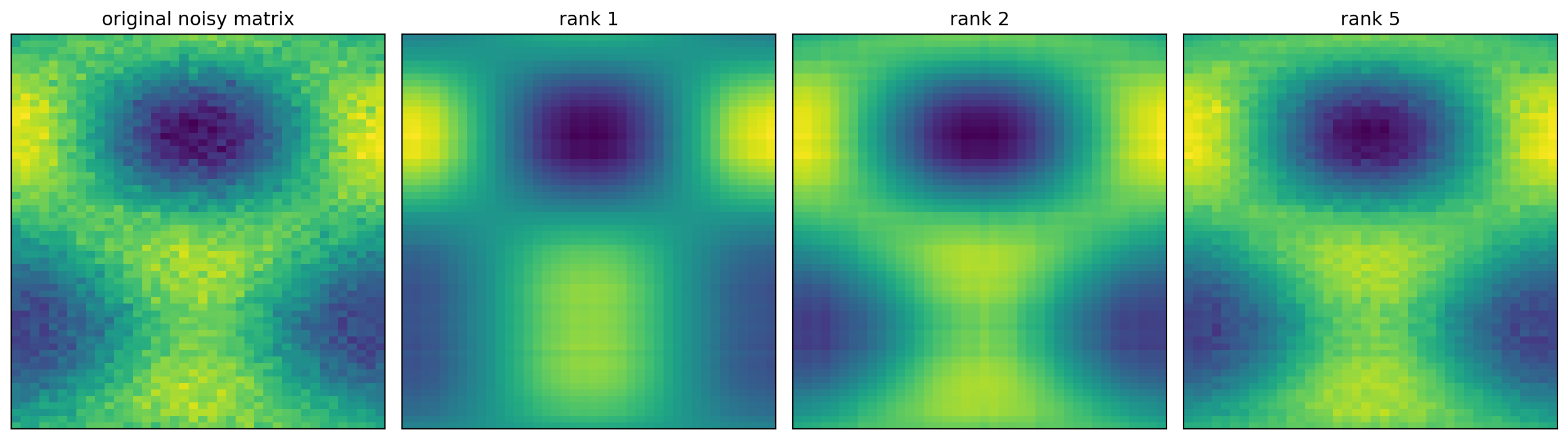
The approximation improves as \(k\) increases.
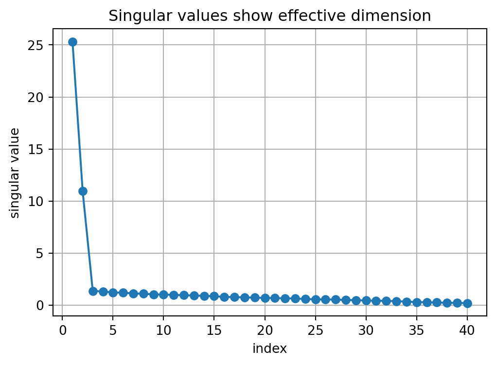
21.26 Python plot: singular values
= (6 , 4 ))1 , len (s)+ 1 ), s, marker= "o" )"index" )"singular value" )True )"Singular values show effective dimension" )
A rapid drop in singular values suggests that the matrix is well approximated by a low-rank matrix.
21.27 Python plot: low-rank approximations
= plt.subplots(1 , 4 , figsize= (14 , 4 ))for ax, M, title in zip ("original noisy matrix" , "rank 1" , "rank 2" , "rank 5" ]= ax.imshow(M, aspect= "auto" )
Low-rank approximations capture the main patterns using fewer components.
21.28 Image compression with SVD
A grayscale image can be represented as a matrix.
If the image matrix is \(A\) , then its SVD is
\[
A=U\Sigma V^T.
\]
A rank-\(k\) approximation is
\[
A_k=\sum_{i=1}^k \sigma_i u_iv_i^T.
\]
Instead of storing all \(mn\) pixel values, we store:
the first \(k\) left singular vectors,
the first \(k\) singular values,
the first \(k\) right singular vectors.
The storage is approximately
\[
k(m+n+1)
\]
numbers instead of
\[
mn.
\]
This can be much smaller when \(k\) is small.
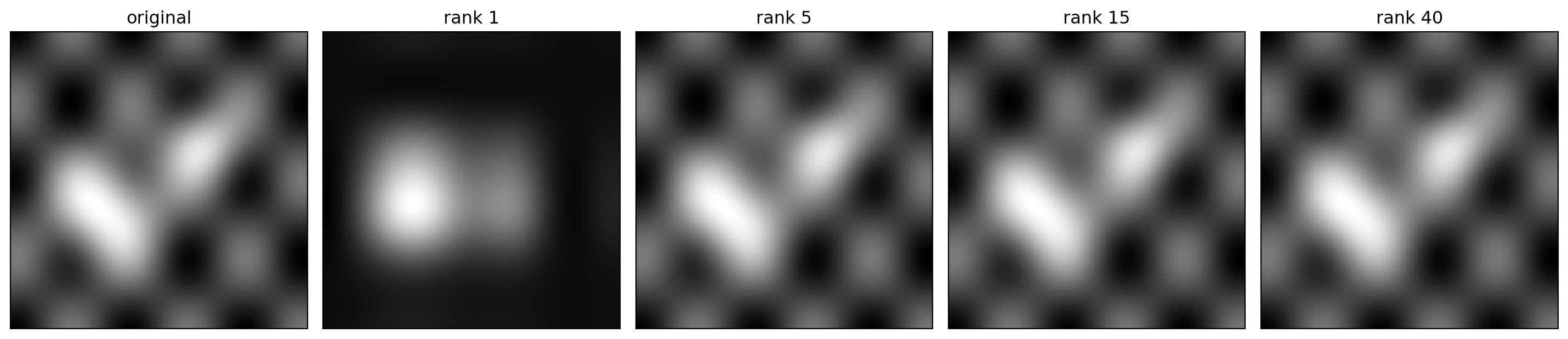
21.29 Python: synthetic image compression
# Create a synthetic grayscale image matrix = 120 = np.linspace(- 1 , 1 , n)= np.linspace(- 1 , 1 , n)= np.meshgrid(x, y)= (- 8 * ((X+ 0.35 )** 2 + (Y- 0.2 )** 2 ))+ 0.8 * np.exp(- 14 * ((X- 0.3 )** 2 + (Y+ 0.25 )** 2 ))+ 0.3 * np.sin(8 * X)* np.cos(6 * Y)= np.linalg.svd(image, full_matrices= False )= [1 , 5 , 15 , 40 ]= plt.subplots(1 , len (ranks) + 1 , figsize= (15 , 4 ))0 ].imshow(image, cmap= "gray" )0 ].set_title("original" )0 ].set_xticks([])0 ].set_yticks([])for ax, k in zip (axes[1 :], ranks):= truncated_svd(U, s, Vt, k)= "gray" )f"rank { k} " )
This demonstrates the idea of image compression using singular values.
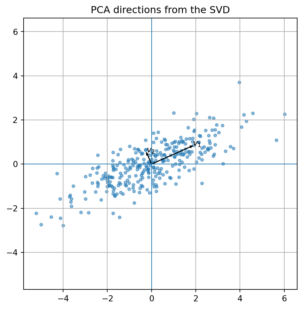
21.30 SVD and PCA
Principal component analysis is based on the SVD.
Suppose \(X\) is a centered data matrix whose rows are observations and columns are features.
The covariance matrix is
\[
C=\frac{1}{m-1}X^TX.
\]
If
\[
X=U\Sigma V^T,
\]
then
\[
X^TX=V\Sigma^T\Sigma V^T.
\]
Thus the right singular vectors of \(X\) are eigenvectors of the covariance matrix.
These are the principal component directions.
The singular values determine explained variance.
Specifically, variances along principal components are proportional to
\[
\sigma_i^2.
\]
21.31 Python: PCA with SVD
= np.random.default_rng(1 )= rng.multivariate_normal(= [0 , 0 ],= [[4 , 1.5 ], [1.5 , 1 ]],= 300 = X - X.mean(axis= 0 )= np.linalg.svd(X_centered, full_matrices= False )= Vt.T= s** 2 / (len (X_centered) - 1 )= (6 , 6 ))0 ], X_centered[:, 1 ], s= 12 , alpha= 0.5 )for i in range (2 ):= principal_directions[:, i]= np.sqrt(explained_variance[i])0 , 0 , length* direction[0 ], length* direction[1 ],= 0.08 , length_includes_head= True )* direction[0 ], length* direction[1 ], f"$v_ { i+ 1 } $" )0 , linewidth= 0.8 )0 , linewidth= 0.8 )True )"equal" )"PCA directions from the SVD" )
array([4.1669323 , 0.33866442])
21.32 SVD and least squares
The SVD also solves least-squares problems.
If
\[
A=U\Sigma V^T,
\]
then a least-squares solution can be written using the pseudoinverse
\[
A^+=V\Sigma^+U^T.
\]
Here \(\Sigma^+\) is formed by replacing each nonzero singular value \(\sigma_i\) with \(1/\sigma_i\) and transposing the diagonal-shaped matrix.
Then the minimum-norm least-squares solution is
\[
\hat x=A^+b.
\]
The SVD pseudoinverse gives
\[
\hat x=A^+b,
\]
where
\[
A^+=V\Sigma^+U^T.
\]
This works even when \(A\) is rectangular or rank deficient.
21.33 Python: pseudoinverse
= np.array([1 , 2 ],2 , 4 ],3 , 6 ]= float )= np.array([1 , 2 , 2 ], dtype= float )= np.linalg.pinv(A) @ b= np.linalg.lstsq(A, b, rcond= None )[0 ]
(array([0.15714286, 0.31428571]), array([0.15714286, 0.31428571]))
The pseudoinverse returns the minimum-norm least-squares solution.
21.34 SVD and noise reduction
If small singular values correspond mostly to noise, then truncated SVD can denoise data.
The idea is:
compute the SVD,
keep the largest singular values,
discard small singular values,
reconstruct the matrix.
This is used in signal processing, recommendation systems, image processing, and latent semantic analysis.
The challenge is choosing how many singular values to keep.
Common strategies include:
look for a spectral gap,
keep enough singular values to explain a desired fraction of energy,
cross-validate performance,
use domain knowledge.
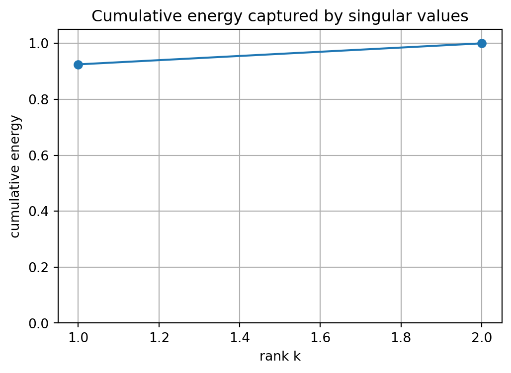
21.35 Energy captured by singular values
The Frobenius norm satisfies
\[
\|A\|_F^2=\sigma_1^2+\cdots+\sigma_r^2.
\]
The fraction of energy captured by the first \(k\) singular values is
\[
\frac{\sigma_1^2+\cdots+\sigma_k^2}{\sigma_1^2+\cdots+\sigma_r^2}.
\]
= np.cumsum(s** 2 ) / np.sum (s** 2 )= (6 , 4 ))1 , len (energy)+ 1 ), energy, marker= "o" )"rank k" )"cumulative energy" )0 , 1.05 )True )"Cumulative energy captured by singular values" )
21.36 Algorithmic summary
For small examples:
Compute
\[
A^TA.
\]
Find eigenvalues
\[
\lambda_i
\]
of \(A^TA\) . 3. Singular values are
\[
\sigma_i=\sqrt{\lambda_i}.
\]
Right singular vectors are eigenvectors of \(A^TA\) .
For \(\sigma_i>0\) , compute
\[
u_i=\frac{Av_i}{\sigma_i}.
\]
Use:
= np.linalg.svd(A, full_matrices= False )Then \(A\) is reconstructed by:
Given
\[
A=U\Sigma V^T,
\]
keep the first \(k\) singular values and vectors:
\[
A_k=U_k\Sigma_kV_k^T.
\]
Given
\[
A=U\Sigma V^T,
\]
form
\[
A^+=V\Sigma^+U^T.
\]
Then the minimum-norm least-squares solution is
\[
\hat x=A^+b.
\]
21.37 Common mistakes
Mistake 1: thinking SVD is only for square matrices
The SVD works for every matrix.
Mistake 2: confusing eigenvalues with singular values
Eigenvalues may be negative or complex.
Singular values are always real and nonnegative.
Mistake 3: forgetting that \(U\) and \(V\) live in different spaces
For an \(m\times n\) matrix:
left singular vectors \(u_i\) live in \(\mathbb{R}^m\) ,
right singular vectors \(v_i\) live in \(\mathbb{R}^n\) .
Mistake 4: using singular values without sorting
Numerical software usually returns singular values in decreasing order, but always check documentation and preserve the corresponding vectors.
Mistake 5: keeping too few singular values
Low-rank approximation is useful, but keeping too few components may lose important structure.
Mistake 6: keeping too many singular values
Keeping very small singular values can preserve noise and numerical instability.
21.38 Chapter summary
The singular value decomposition writes any matrix as
\[
A=U\Sigma V^T.
\]
The right singular vectors \(v_i\) are input directions.
The left singular vectors \(u_i\) are output directions.
The singular values \(\sigma_i\) are nonnegative stretching factors satisfying
\[
Av_i=\sigma_i u_i.
\]
The singular values are square roots of eigenvalues of \(A^TA\) .
The rank of \(A\) is the number of nonzero singular values.
The SVD gives orthonormal bases for the four fundamental subspaces.
The outer product form is
\[
A=\sum_{i=1}^r \sigma_i u_iv_i^T.
\]
The truncated SVD
\[
A_k=\sum_{i=1}^k \sigma_i u_iv_i^T
\]
is the best rank-\(k\) approximation.
The SVD supports image compression, PCA, denoising, least squares, pseudoinverses, and many AI algorithms.
Exercises
A. Singular values from \(A^TA\)
For each matrix, compute \(A^TA\) , find its eigenvalues, and determine the singular values.
\[
A=
\begin{bmatrix}
3&0\\
0&1
\end{bmatrix}
\]
\[
A=
\begin{bmatrix}
0&2\\
3&0
\end{bmatrix}
\]
\[
A=
\begin{bmatrix}
1&0\\
0&0
\end{bmatrix}
\]
\[
A=
\begin{bmatrix}
1&2\\
2&4\\
3&6
\end{bmatrix}
\]
B. Singular vector relations
For
\[
A=
\begin{bmatrix}
2&1\\
0&1
\end{bmatrix},
\]
Compute the SVD using Python.
Verify that
\[
Av_i=\sigma_i u_i.
\]
Verify that
\[
A^TAv_i=\sigma_i^2v_i.
\]
C. Rank and condition number
For each matrix:
Compute singular values.
Determine the rank.
If the matrix is square and invertible, compute the condition number.
Matrices:
\[
\begin{bmatrix}
2&0\\
0&1
\end{bmatrix},
\quad
\begin{bmatrix}
1&0\\
0&0.001
\end{bmatrix},
\quad
\begin{bmatrix}
1&2\\
2&4
\end{bmatrix}.
\]
D. Low-rank approximation
Let
\[
A=
\begin{bmatrix}
3&2&0\\
2&3&0\\
0&0&1
\end{bmatrix}.
\]
Compute the SVD.
Construct the rank-\(1\) approximation.
Construct the rank-\(2\) approximation.
Compare approximation errors.
E. Four fundamental subspaces
For a rank-deficient matrix of your choice:
Compute the SVD.
Identify bases for \(\operatorname{Col}(A)\) .
Identify bases for \(\operatorname{Row}(A)\) .
Identify bases for \(\operatorname{Null}(A)\) .
Identify bases for \(\operatorname{Null}(A^T)\) .
F. Image compression
Create or load a grayscale image matrix.
Compute its SVD.
Reconstruct rank-\(5\) , rank-\(20\) , and rank-\(50\) approximations.
Compare visual quality.
Compute storage savings.
G. PCA using SVD
Generate a two-dimensional data set.
Center the data.
Compute the SVD.
Plot the right singular vectors as principal directions.
Compute explained variance from singular values.
H. Python exercises
Write a function that computes a rank-\(k\) truncated SVD approximation.
Plot singular values of a matrix.
Plot cumulative energy captured by singular values.
Compare np.linalg.svd, np.linalg.matrix_rank, and np.linalg.cond.
Use np.linalg.pinv to solve a rank-deficient least-squares problem.
Use SVD to denoise a noisy matrix.
I. Reflection
Write a short paragraph answering each question.
Why does the SVD work for rectangular matrices while eigenvalue decomposition does not?
Why are singular values always nonnegative?
How does the SVD describe the geometry of a matrix?
Why is truncated SVD useful for compression?
Why is the SVD central in data science and AI?
AI-age connection
The SVD is one of the most important tools in modern data science and AI. It identifies dominant directions in data, compresses images, denoises signals, solves least-squares problems, computes pseudoinverses, and provides the foundation for PCA. In high-dimensional learning, singular values reveal effective dimension, numerical rank, conditioning, and hidden low-rank structure. The SVD is the language of linear structure inside large data matrices.