Opening question
Eigenvectors reveal directions that a matrix does not turn.
If a matrix has enough eigenvectors to form a basis, then the matrix becomes simple in that basis. Instead of mixing coordinates, it only scales them.
This is the idea of diagonalization .
A diagonal matrix is easy to understand:
\[
D=
\begin{bmatrix}
\lambda_1&0&\cdots&0\\
0&\lambda_2&\cdots&0\\
\vdots&\vdots&\ddots&\vdots\\
0&0&\cdots&\lambda_n
\end{bmatrix}.
\]
It acts by
\[
Dx=
\begin{bmatrix}
\lambda_1x_1\\
\lambda_2x_2\\
\vdots\\
\lambda_nx_n
\end{bmatrix}.
\]
So each coordinate evolves independently.
The central question of this chapter is:
When can we choose coordinates so that a matrix becomes diagonal?
This question is especially powerful for systems that evolve by repeated multiplication:
\[
x_{k+1}=Ax_k.
\]
Such systems are called discrete dynamical systems .
Learning goals
After studying this chapter, you should be able to:
Define diagonalization.
Determine whether a matrix is diagonalizable.
Construct matrices \(P\) and \(D\) from eigenvectors and eigenvalues.
Use diagonalization to compute powers \(A^k\) .
Solve discrete dynamical systems \(x_{k+1}=Ax_k\) .
Interpret long-term behavior using eigenvalues.
Understand stable, unstable, and neutral directions.
Analyze simple Markov chains and steady states.
Use Python to compute diagonalizations and simulate dynamics.
Connect diagonalization to data, ranking, iteration, and AI.
18.1 Why diagonal matrices are simple
Let
\[
D=
\begin{bmatrix}
3&0\\
0&1
\end{bmatrix}.
\]
Then
\[
D
\begin{bmatrix}
x\\
y
\end{bmatrix}
=
\begin{bmatrix}
3x\\
y
\end{bmatrix}.
\]
The first coordinate is multiplied by \(3\) .
The second coordinate is multiplied by \(1\) .
There is no mixing between coordinates.
Powers of diagonal matrices are also simple:
\[
D^k=
\begin{bmatrix}
3^k&0\\
0&1^k
\end{bmatrix}.
\]
More generally, if
\[
D=\operatorname{diag}(\lambda_1,\ldots,\lambda_n),
\]
then
\[
D^k=\operatorname{diag}(\lambda_1^k,\ldots,\lambda_n^k).
\]
If
\[
D=\operatorname{diag}(\lambda_1,\ldots,\lambda_n),
\]
then
\[
D^k=\operatorname{diag}(\lambda_1^k,\ldots,\lambda_n^k).
\]
This is the main reason diagonalization is useful.
18.2 Eigenvector coordinates
Suppose \(A\) has eigenvectors
\[
v_1,\ldots,v_n
\]
that form a basis of \(\mathbb{R}^n\) , with corresponding eigenvalues
\[
\lambda_1,\ldots,\lambda_n.
\]
Then every vector \(x\) can be written uniquely as
\[
x=c_1v_1+\cdots+c_nv_n.
\]
Applying \(A\) gives
\[
Ax=c_1Av_1+\cdots+c_nAv_n.
\]
Since
\[
Av_j=\lambda_jv_j,
\]
we get
\[
Ax=c_1\lambda_1v_1+\cdots+c_n\lambda_nv_n.
\]
So in the eigenvector basis, \(A\) simply scales each coordinate.
This is diagonalization.
18.4 Example: diagonalizing a \(2\times 2\) matrix
Let
\[
A=
\begin{bmatrix}
2&1\\
1&2
\end{bmatrix}.
\]
From the previous chapter, eigenvectors and eigenvalues are:
\[
v_1=
\begin{bmatrix}
1\\
1
\end{bmatrix},
\qquad
\lambda_1=3,
\]
and
\[
v_2=
\begin{bmatrix}
1\\
-1
\end{bmatrix},
\qquad
\lambda_2=1.
\]
Thus
\[
P=
\begin{bmatrix}
1&1\\
1&-1
\end{bmatrix},
\qquad
D=
\begin{bmatrix}
3&0\\
0&1
\end{bmatrix}.
\]
Then
\[
A=PDP^{-1}.
\]
This says that \(A\) becomes diagonal in the basis
\[
\left\{
\begin{bmatrix}
1\\
1
\end{bmatrix},
\begin{bmatrix}
1\\
-1
\end{bmatrix}
\right\}.
\]
18.5 Python: checking diagonalization
import numpy as npimport matplotlib.pyplot as plt= np.array([[2 , 1 ],1 , 2 ]], dtype= float )= np.array([[1 , 1 ],1 , - 1 ]], dtype= float )= np.array([[3 , 0 ],0 , 1 ]], dtype= float )@ D @ np.linalg.inv(P), A
(array([[2., 1.],
        [1., 2.]]),
 array([[2., 1.],
        [1., 2.]]))
Check the coordinate version:
array([[3., 0.],
       [0., 1.]])
This should equal \(D\) up to numerical roundoff.
18.6 When is a matrix diagonalizable?
An \(n\times n\) matrix is diagonalizable if it has \(n\) linearly independent eigenvectors.
An \(n\times n\) matrix \(A\) is diagonalizable if and only if \(A\) has a basis of \(\mathbb{R}^n\) consisting of eigenvectors.
A useful sufficient condition is:
If an \(n\times n\) matrix has \(n\) distinct eigenvalues, then it is diagonalizable.
Why?
Eigenvectors corresponding to distinct eigenvalues are linearly independent.
However, a matrix can still be diagonalizable even if some eigenvalues repeat, as long as it has enough independent eigenvectors.
18.7 A matrix that is not diagonalizable
Consider
\[
A=
\begin{bmatrix}
2&1\\
0&2
\end{bmatrix}.
\]
The only eigenvalue is
\[
\lambda=2
\]
with algebraic multiplicity \(2\) .
Compute
\[
A-2I=
\begin{bmatrix}
0&1\\
0&0
\end{bmatrix}.
\]
Solving
\[
(A-2I)v=0
\]
gives
\[
v=
\begin{bmatrix}
x\\
0
\end{bmatrix}.
\]
So the eigenspace is
\[
E_2=\operatorname{span}
\left\{
\begin{bmatrix}
1\\
0
\end{bmatrix}
\right\}.
\]
There is only one independent eigenvector.
Since a \(2\times 2\) matrix needs two independent eigenvectors to be diagonalizable, this matrix is not diagonalizable.
18.8 Algebraic and geometric multiplicity
Recall:
algebraic multiplicity is multiplicity as a root of the characteristic polynomial,
geometric multiplicity is the dimension of the eigenspace.
For an eigenvalue \(\lambda\) ,
\[
1\le \dim(E_\lambda)\le \text{algebraic multiplicity of }\lambda.
\]
A matrix is diagonalizable if the total number of independent eigenvectors is \(n\) .
Equivalently, for each eigenvalue, the geometric multiplicity must add up correctly so that all eigenspaces together provide \(n\) independent directions.
18.9 Algorithm for diagonalizing a matrix
To diagonalize an \(n\times n\) matrix \(A\) :
Find the eigenvalues by solving
\[
\det(A-\lambda I)=0.
\]
For each eigenvalue \(\lambda\) , find a basis for
\[
E_\lambda=\operatorname{Null}(A-\lambda I).
\]
If the total number of independent eigenvectors is \(n\) , form
\[
P=\begin{bmatrix}v_1&v_2&\cdots&v_n\end{bmatrix}.
\]
Form
\[
D=\operatorname{diag}(\lambda_1,\ldots,\lambda_n)
\]
in the same order as the columns of \(P\) . 5. Then
\[
A=PDP^{-1}.
\]
The ordering matters: the \(j\) th diagonal entry of \(D\) must correspond to the \(j\) th column of \(P\) .
18.10 Powers of diagonalizable matrices
If
\[
A=PDP^{-1},
\]
then
\[
A^2=(PDP^{-1})(PDP^{-1})=PD^2P^{-1}.
\]
Similarly,
\[
A^k=PD^kP^{-1}.
\]
Since powers of diagonal matrices are easy,
\[
D^k=\operatorname{diag}(\lambda_1^k,\ldots,\lambda_n^k).
\]
If
\[
A=PDP^{-1},
\]
then
\[
A^k=PD^kP^{-1}.
\]
This formula is one of the main applications of diagonalization.
18.11 Example: computing \(A^k\)
Let
\[
A=
\begin{bmatrix}
2&1\\
1&2
\end{bmatrix}.
\]
We have
\[
A=PDP^{-1},
\]
where
\[
P=
\begin{bmatrix}
1&1\\
1&-1
\end{bmatrix},
\qquad
D=
\begin{bmatrix}
3&0\\
0&1
\end{bmatrix}.
\]
Therefore
\[
A^k
=
P
\begin{bmatrix}
3^k&0\\
0&1
\end{bmatrix}
P^{-1}.
\]
Since
\[
P^{-1}
=
\frac12
\begin{bmatrix}
1&1\\
1&-1
\end{bmatrix},
\]
we get
\[
A^k
=
\frac12
\begin{bmatrix}
1&1\\
1&-1
\end{bmatrix}
\begin{bmatrix}
3^k&0\\
0&1
\end{bmatrix}
\begin{bmatrix}
1&1\\
1&-1
\end{bmatrix}.
\]
Multiplying gives
\[
A^k
=
\frac12
\begin{bmatrix}
3^k+1&3^k-1\\
3^k-1&3^k+1
\end{bmatrix}.
\]
18.12 Python: powers by diagonalization
def power_by_diagonalization(P, D, k):return P @ np.linalg.matrix_power(D, k) @ np.linalg.inv(P)for k in range (1 , 5 ):print ("k =" , k)print (power_by_diagonalization(P, D, k))print (np.linalg.matrix_power(A, k))print ()
k = 1
[[2. 1.]
 [1. 2.]]
[[2. 1.]
 [1. 2.]]

k = 2
[[5. 4.]
 [4. 5.]]
[[5. 4.]
 [4. 5.]]

k = 3
[[14. 13.]
 [13. 14.]]
[[14. 13.]
 [13. 14.]]

k = 4
[[41. 40.]
 [40. 41.]]
[[41. 40.]
 [40. 41.]]
The two methods agree up to numerical roundoff.
18.13 Discrete dynamical systems
A discrete dynamical system evolves step by step:
\[
x_{k+1}=Ax_k.
\]
Starting from an initial vector \(x_0\) , we get
\[
x_1=Ax_0,
\]
\[
x_2=A^2x_0,
\]
and in general,
\[
x_k=A^kx_0.
\]
If \(A\) is diagonalizable,
\[
x_k=PD^kP^{-1}x_0.
\]
This formula explains the long-term behavior of the system.
18.14 Dynamics in eigenvector coordinates
Suppose \(A\) has eigenvectors \(v_1,\ldots,v_n\) and eigenvalues \(\lambda_1,\ldots,\lambda_n\) .
Write the initial vector as
\[
x_0=c_1v_1+\cdots+c_nv_n.
\]
Then
\[
x_k=A^kx_0=c_1\lambda_1^kv_1+\cdots+c_n\lambda_n^kv_n.
\]
Each eigenvector direction evolves independently.
If
\[
x_0=c_1v_1+\cdots+c_nv_n,
\]
then
\[
x_k=A^kx_0=c_1\lambda_1^kv_1+\cdots+c_n\lambda_n^kv_n.
\]
This is the main interpretation of diagonalization for dynamics.
18.15 Stability from eigenvalues
For the system
\[
x_{k+1}=Ax_k,
\]
eigenvalues determine growth or decay.
For an eigen-direction \(v\) with eigenvalue \(\lambda\) ,
\[
A^kv=\lambda^kv.
\]
Therefore:
If \(|\lambda|<1\) , that direction decays to zero.
If \(|\lambda|>1\) , that direction grows.
If \(\lambda=1\) , that direction remains constant.
If \(\lambda=-1\) , that direction alternates sign.
If \(\lambda<0\) , that direction flips sign each step.
If \(\lambda\) is complex, behavior may oscillate.
For discrete dynamics, \(|\lambda|\) controls growth or decay.
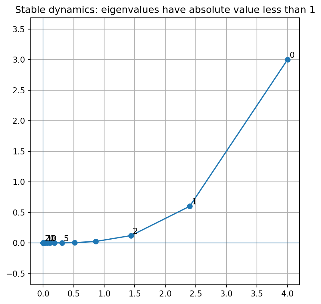
18.16 Example: stable system
Let
\[
A=
\begin{bmatrix}
0.6&0\\
0&0.2
\end{bmatrix}.
\]
Then
\[
x_{k+1}=Ax_k
\]
has eigenvalues
\[
0.6
\]
and
\[
0.2.
\]
Both have absolute value less than \(1\) .
Therefore every trajectory tends to zero.
= np.array([[0.6 , 0 ],0 , 0.2 ]], dtype= float )= np.array([4 , 3 ], dtype= float )= [x.copy()]for k in range (20 ):= A_stable @ x= np.array(points)= (6 , 6 ))0 ], points[:, 1 ], marker= "o" )for k in [0 , 1 , 2 , 5 , 10 , 20 ]:0 ] + 0.03 , points[k, 1 ] + 0.03 , str (k))0 , linewidth= 0.8 )0 , linewidth= 0.8 )True )"equal" )"Stable dynamics: eigenvalues have absolute value less than 1" )
18.17 Example: unstable system
Let
\[
A=
\begin{bmatrix}
1.2&0\\
0&0.8
\end{bmatrix}.
\]
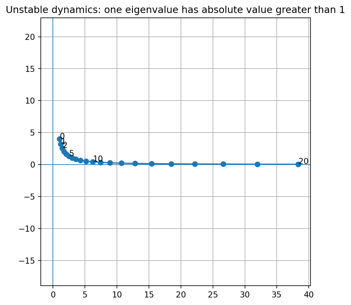
The eigenvalue \(1.2\) causes growth in the first coordinate.
The eigenvalue \(0.8\) causes decay in the second coordinate.
Most initial vectors eventually align with the growing eigen-direction.
= np.array([[1.2 , 0 ],0 , 0.8 ]], dtype= float )= np.array([1 , 4 ], dtype= float )= [x.copy()]for k in range (20 ):= A_unstable @ x= np.array(points)= (6 , 6 ))0 ], points[:, 1 ], marker= "o" )for k in [0 , 1 , 2 , 5 , 10 , 20 ]:0 ] + 0.03 , points[k, 1 ] + 0.03 , str (k))0 , linewidth= 0.8 )0 , linewidth= 0.8 )True )"equal" )"Unstable dynamics: one eigenvalue has absolute value greater than 1" )
18.18 Example: diagonalizable dynamics with mixed directions
Let
\[
A=
\begin{bmatrix}
2&1\\
1&2
\end{bmatrix}.
\]
The eigenvectors are
\[
v_1=\begin{bmatrix}1\\1\end{bmatrix},
\qquad
v_2=\begin{bmatrix}1\\-1\end{bmatrix},
\]
with eigenvalues \(3\) and \(1\) .
Let
\[
x_0=
\begin{bmatrix}
2\\
0
\end{bmatrix}.
\]
Then
\[
x_0=v_1+v_2.
\]
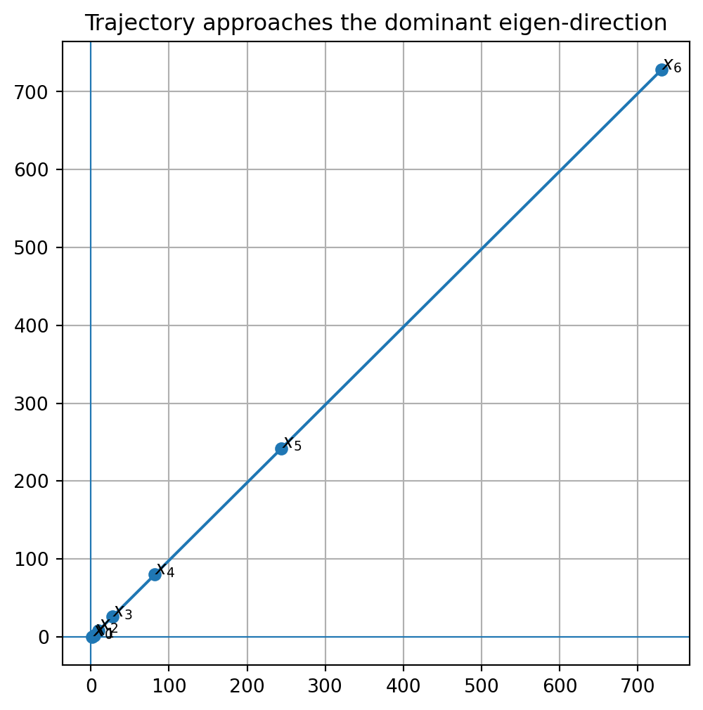
So
\[
x_k=3^kv_1+1^kv_2.
\]
As \(k\) grows, the \(v_1\) direction dominates.
= np.array([[2 , 1 ],1 , 2 ]], dtype= float )= np.array([2 , 0 ], dtype= float )= [x.copy()]for k in range (6 ):= A @ x= np.array(points)= (6 , 6 ))0 ], points[:, 1 ], marker= "o" )for k, p in enumerate (points):0 ] + 0.1 , p[1 ] + 0.1 , f"$x_ { k} $" )0 , linewidth= 0.8 )0 , linewidth= 0.8 )True )"equal" )"Trajectory approaches the dominant eigen-direction" )
18.19 Long-term behavior and dominant eigenvalues
An eigenvalue with largest absolute value is called a dominant eigenvalue .
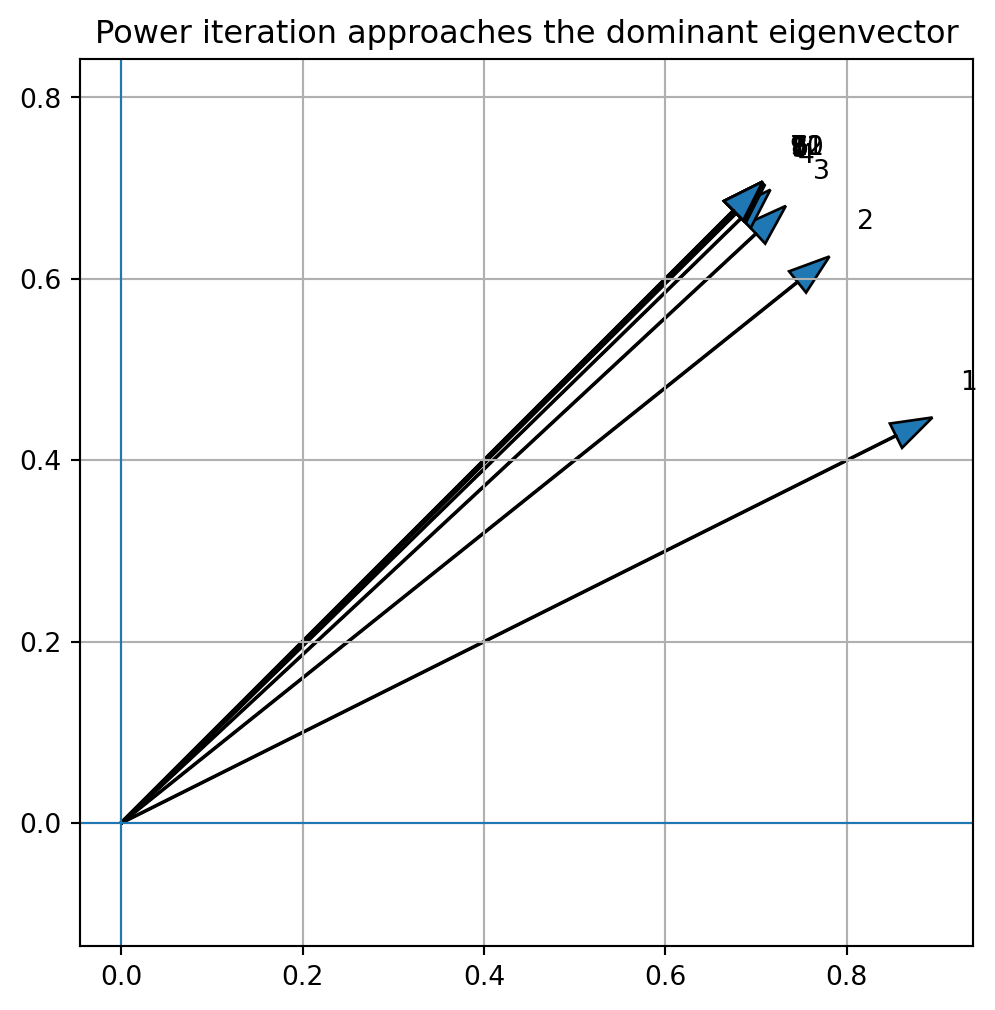
If one eigenvalue has strictly largest absolute value and the initial vector has a component in its eigenvector direction, then repeated multiplication tends to align with the dominant eigenvector.
This idea is behind power iteration , a simple method for computing dominant eigenvectors.
It also appears in ranking algorithms, Markov chains, population models, and graph algorithms.
18.20 Power iteration
Power iteration repeatedly applies a matrix and normalizes:
\[
y_k=Ax_k,
\]
\[
x_{k+1}=\frac{y_k}{\|y_k\|}.
\]
If the conditions are favorable, \(x_k\) approaches a dominant eigenvector direction.
= np.array([[2 , 1 ],1 , 2 ]], dtype= float )= np.array([1 , 0 ], dtype= float )= []for k in range (12 ):= A @ x= y / np.linalg.norm(y)
array([[0.89442719, 0.4472136 ],
       [0.78086881, 0.62469505],
       [0.73279349, 0.6804511 ],
       [0.71578195, 0.69832385],
       [0.71001067, 0.70419091],
       [0.70807608, 0.70613615],
       [0.70743003, 0.70678338],
       [0.70721455, 0.706999  ],
       [0.70714271, 0.70707086],
       [0.70711876, 0.70709481],
       [0.70711077, 0.70710279],
       [0.70710811, 0.70710545]])
= np.array(history)= (6 , 6 ))for k, v in enumerate (history):0 , 0 , v[0 ], v[1 ], head_width= 0.03 , length_includes_head= True )0 ] + 0.03 , v[1 ] + 0.03 , str (k+ 1 ))0 , linewidth= 0.8 )0 , linewidth= 0.8 )True )"equal" )"Power iteration approaches the dominant eigenvector" )
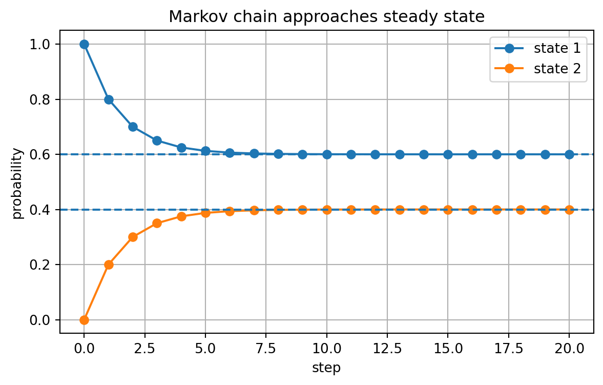
18.21 Markov chains as dynamical systems
A simple Markov chain can be written as
\[
x_{k+1}=Px_k,
\]
where \(x_k\) is a probability vector and \(P\) is a transition matrix.
For example,
\[
P=
\begin{bmatrix}
0.8&0.3\\
0.2&0.7
\end{bmatrix}.
\]
The columns of \(P\) add to \(1\) , so if \(x_k\) is a probability vector, then \(x_{k+1}\) is also a probability vector.
A steady state is a vector \(\pi\) satisfying
\[
P\pi=\pi.
\]
This is an eigenvector equation with eigenvalue \(1\) .
18.22 Example: steady state
Let
\[
P=
\begin{bmatrix}
0.8&0.3\\
0.2&0.7
\end{bmatrix}.
\]
We want
\[
P\pi=\pi.
\]
That is,
\[
(P-I)\pi=0.
\]
Also, since \(\pi\) is a probability vector,
\[
\pi_1+\pi_2=1.
\]
Solve:
\[
\begin{bmatrix}
-0.2&0.3\\
0.2&-0.3
\end{bmatrix}
\begin{bmatrix}
\pi_1\\
\pi_2
\end{bmatrix}
=0.
\]
The first equation is
\[
-0.2\pi_1+0.3\pi_2=0.
\]
So
\[
0.3\pi_2=0.2\pi_1.
\]
Thus
\[
3\pi_2=2\pi_1.
\]
Together with
\[
\pi_1+\pi_2=1,
\]
we get
\[
\pi_1=\frac35,
\qquad
\pi_2=\frac25.
\]
So
\[
\pi=
\begin{bmatrix}
3/5\\
2/5
\end{bmatrix}.
\]
18.23 Python: Markov chain iteration
= np.array([[0.8 , 0.3 ],0.2 , 0.7 ]], dtype= float )= np.array([1.0 , 0.0 ])= [x.copy()]for k in range (20 ):= P @ x= np.array(history)= (7 , 4 ))0 ], marker= "o" , label= "state 1" )1 ], marker= "o" , label= "state 2" )3 / 5 , linestyle= "--" )2 / 5 , linestyle= "--" )"step" )"probability" )True )"Markov chain approaches steady state" )- 1 ]
array([0.60000038, 0.39999962])
The probabilities approach the eigenvector with eigenvalue \(1\) .
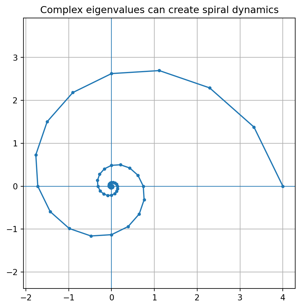
18.24 Complex eigenvalues and oscillation preview
Some real matrices have complex eigenvalues.
For example, a rotation matrix
\[
R_\theta=
\begin{bmatrix}
\cos\theta&-\sin\theta\\
\sin\theta&\cos\theta
\end{bmatrix}
\]
has complex eigenvalues
\[
e^{i\theta}
\]
and
\[
e^{-i\theta}.
\]
Repeated multiplication rotates vectors.
If the eigenvalues have magnitude \(1\) , motion may persist.
If the eigenvalues have magnitude less than \(1\) , motion spirals inward.
If they have magnitude greater than \(1\) , motion spirals outward.
This connects eigenvalues to oscillation and stability.
18.25 Python: spiral dynamics
= np.pi / 8 = 0.9 = scale * np.array([- np.sin(theta)],= np.array([4.0 , 0.0 ])= [x.copy()]for k in range (60 ):= A_spiral @ x= np.array(points)= (6 , 6 ))0 ], points[:, 1 ], marker= "o" , markersize= 3 )0 , linewidth= 0.8 )0 , linewidth= 0.8 )True )"equal" )"Complex eigenvalues can create spiral dynamics" )
18.26 Change of basis interpretation
Diagonalization is a special case of change of basis.
The matrix
\[
P^{-1}AP=D
\]
means:
use \(P^{-1}\) to convert a vector into eigenvector coordinates,
apply the diagonal matrix \(D\) ,
use \(P\) to convert back to standard coordinates.
So diagonalization says:
In the right coordinate system, the transformation separates into independent one-dimensional actions.
This is why eigenvectors are powerful. They give the coordinate system that the matrix itself prefers.
18.27 Computational caution
Diagonalization is conceptually powerful, but not always the best numerical method.
Reasons:
A matrix may not be diagonalizable.
Eigenvector matrices can be ill-conditioned.
Repeated eigenvalues can be sensitive to perturbations.
Numerical algorithms use stable factorizations depending on the task.
For symmetric matrices, eigenvalue computations are especially well-behaved because eigenvectors can be chosen orthonormally. This leads to the spectral theorem, one of the central results of linear algebra.
18.28 Python: diagonalization with NumPy
= np.array([[2 , 1 ],1 , 2 ]], dtype= float )= np.linalg.eig(A)= np.diag(eigvals)= P @ D @ np.linalg.inv(P)
(array([3., 1.]),
 array([[ 0.70710678, -0.70710678],
        [ 0.70710678,  0.70710678]]),
 array([[3., 0.],
        [0., 1.]]),
 array([[2., 1.],
        [1., 2.]]))
Measure reconstruction error:
- reconstructed)
For a non-diagonalizable matrix, NumPy may still return eigenvalues and some eigenvectors, but the eigenvector matrix may be singular or poorly conditioned.
= np.array([[2 , 1 ],0 , 2 ]], dtype= float )= np.linalg.eig(B)
(array([2., 2.]),
 array([[ 1.0000000e+00, -1.0000000e+00],
        [ 0.0000000e+00,  4.4408921e-16]]),
 4.4408920985006143e-16)
The determinant of the eigenvector matrix is close to zero, reflecting that there are not enough independent eigenvectors.
18.29 Algorithmic summary
Given an \(n\times n\) matrix \(A\) :
Find all eigenvalues.
Find a basis for each eigenspace.
Count the total number of independent eigenvectors.
If there are \(n\) independent eigenvectors, \(A\) is diagonalizable.
If not, \(A\) is not diagonalizable.
If \(A\) has \(n\) independent eigenvectors:
Put eigenvectors into columns of \(P\) .
Put corresponding eigenvalues on the diagonal of \(D\) in the same order.
Then
\[
A=PDP^{-1}.
\]
If
\[
A=PDP^{-1},
\]
then
\[
A^k=PD^kP^{-1}.
\]
For
\[
x_{k+1}=Ax_k,
\]
we have
\[
x_k=A^kx_0.
\]
If \(A=PDP^{-1}\) , then
\[
x_k=PD^kP^{-1}x_0.
\]
18.30 Common mistakes
Mistake 1: assuming every matrix is diagonalizable
Not every square matrix has enough eigenvectors.
For example,
\[
\begin{bmatrix}
2&1\\
0&2
\end{bmatrix}
\]
is not diagonalizable.
Mistake 2: putting eigenvalues in the wrong order
The diagonal entries of \(D\) must correspond to the columns of \(P\) .
Mistake 3: forgetting that \(P\) must be invertible
The eigenvectors must be linearly independent.
If \(P\) is singular, then \(A=PDP^{-1}\) is impossible.
Mistake 4: confusing \(PDP^{-1}\) and \(P^{-1}DP\)
The diagonalization formula is
\[
A=PDP^{-1}.
\]
The coordinate-change form is
\[
P^{-1}AP=D.
\]
Mistake 5: using diagonalization when numerical stability matters
Diagonalization is excellent for theory. For numerical computation, use stable algorithms designed for the task.
18.31 Chapter summary
A matrix is diagonalizable if it has a basis of eigenvectors.
If
\[
P=\begin{bmatrix}v_1&\cdots&v_n\end{bmatrix}
\]
and
\[
D=\operatorname{diag}(\lambda_1,\ldots,\lambda_n),
\]
with
\[
Av_j=\lambda_jv_j,
\]
then
\[
A=PDP^{-1}.
\]
Equivalently,
\[
P^{-1}AP=D.
\]
If \(A=PDP^{-1}\) , then
\[
A^k=PD^kP^{-1}.
\]
For a discrete dynamical system
\[
x_{k+1}=Ax_k,
\]
we have
\[
x_k=A^kx_0.
\]
Eigenvalues determine growth, decay, oscillation, and stability.
Markov chain steady states are eigenvectors with eigenvalue \(1\) .
Diagonalization reveals the coordinate system in which a transformation separates into independent directions.
Exercises
A. Diagonalization by hand
For each matrix:
Find eigenvalues.
Find eigenvectors.
Determine whether the matrix is diagonalizable.
If diagonalizable, find \(P\) and \(D\) .
\[
A=
\begin{bmatrix}
2&1\\
1&2
\end{bmatrix}
\]
\[
A=
\begin{bmatrix}
3&0\\
0&2
\end{bmatrix}
\]
\[
A=
\begin{bmatrix}
1&2\\
0&3
\end{bmatrix}
\]
\[
A=
\begin{bmatrix}
2&1\\
0&2
\end{bmatrix}
\]
B. Matrix powers
Use diagonalization to compute \(A^k\) .
\[
A=
\begin{bmatrix}
2&1\\
1&2
\end{bmatrix}
\]
\[
A=
\begin{bmatrix}
3&0\\
0&2
\end{bmatrix}
\]
\[
A=
\begin{bmatrix}
1&2\\
0&3
\end{bmatrix}
\]
C. Discrete dynamics
For each system, describe long-term behavior.
\[
x_{k+1}=
\begin{bmatrix}
0.5&0\\
0&0.25
\end{bmatrix}
x_k.
\]
\[
x_{k+1}=
\begin{bmatrix}
1.2&0\\
0&0.8
\end{bmatrix}
x_k.
\]
\[
x_{k+1}=
\begin{bmatrix}
2&1\\
1&2
\end{bmatrix}
x_k.
\]
\[
x_{k+1}=
\begin{bmatrix}
0&-1\\
1&0
\end{bmatrix}
x_k.
\]
D. Eigenvector coordinates
Let
\[
A=
\begin{bmatrix}
2&1\\
1&2
\end{bmatrix}.
\]
Use eigenvectors
\[
v_1=
\begin{bmatrix}
1\\
1
\end{bmatrix},
\qquad
v_2=
\begin{bmatrix}
1\\
-1
\end{bmatrix}.
\]
Write
\[
x_0=
\begin{bmatrix}
2\\
0
\end{bmatrix}
\]
as a linear combination of \(v_1\) and \(v_2\) .
Find a formula for \(x_k=A^kx_0\) .
Describe the dominant direction.
E. Markov chains
Let
\[
P=
\begin{bmatrix}
0.8&0.3\\
0.2&0.7
\end{bmatrix}.
\]
Verify that columns of \(P\) sum to \(1\) .
Find a steady state \(\pi\) satisfying
\[
P\pi=\pi.
\]
Normalize \(\pi\) so its entries sum to \(1\) .
Starting from
\[
x_0=
\begin{bmatrix}
1\\
0
\end{bmatrix},
\]
compute several iterations and compare with the steady state.
F. Python exercises
Use NumPy to diagonalize a \(2\times 2\) matrix.
Verify that \(A=PDP^{-1}\) .
Compute \(A^k\) using diagonalization and compare with np.linalg.matrix_power.
Simulate a stable system and an unstable system.
Implement power iteration.
Simulate the Markov chain in this chapter.
Explore a rotation-scaling matrix that creates spirals.
G. Reflection
Write a short paragraph answering each question.
Why is diagonalization a change of basis?
Why does an eigenvector basis make a matrix simple?
Why does diagonalization make matrix powers easy?
How do eigenvalues determine stability?
How do diagonalization and dynamics appear in data science and AI?
AI-age connection
Diagonalization explains how repeated linear processes behave. This matters in ranking algorithms, graph methods, Markov chains, recommendation systems, stability analysis, iterative algorithms, and spectral learning. In data science and AI, diagonalization and its relatives reveal dominant directions, long-term behavior, and hidden coordinate systems. The core idea is that a complicated transformation may become simple when expressed in the right basis.