10 Subspaces of \(\mathbb{R}^n\)

10.1 Opening question

In earlier chapters, we studied spans, linear independence, bases, and dimension. These ideas naturally lead to one of the most important objects in linear algebra:

a subspace.

A subspace is a set of vectors that is closed under the operations of linear algebra. If we add vectors in the set, we stay in the set. If we multiply a vector in the set by a scalar, we stay in the set.

Subspaces are the natural habitats of linear algebra.

They appear as:

lines and planes through the origin,
solution sets of homogeneous systems,
spans of vectors,
column spaces of matrices,
nullspaces of matrices,
row spaces of matrices,
spaces of possible outputs,
spaces of invisible inputs.

The central question of this chapter is:

What kinds of sets behave like vector spaces inside \(\mathbb{R}^n\)?

10.2 Learning goals

After studying this chapter, you should be able to:

Define a subspace of \(\mathbb{R}^n\).
Test whether a subset of \(\mathbb{R}^n\) is a subspace.
Recognize spans as subspaces.
Recognize solution sets of homogeneous systems as subspaces.
Understand why nonhomogeneous solution sets are usually not subspaces.
Define the column space, nullspace, and row space of a matrix.
Find bases for column spaces using pivot columns.
Find bases for nullspaces using row reduction.
Use rank and nullity to describe dimensions.
Visualize subspaces in \(\mathbb{R}^2\) and \(\mathbb{R}^3\) using Python.

10.3 8.1 What is a subspace?

Definition: subspace of \(\mathbb{R}^n\)

A subset \(W\) of \(\mathbb{R}^n\) is a subspace of \(\mathbb{R}^n\) if:

\(0\in W\).
If \(u,v\in W\), then \(u+v\in W\).
If \(u\in W\) and \(c\in\mathbb{R}\), then \(cu\in W\).

The three conditions say:

the zero vector is included,
the set is closed under vector addition,
the set is closed under scalar multiplication.

These are exactly the operations used to form linear combinations.

Therefore, if \(W\) is a subspace and \(u,v\in W\), then every linear combination

\[ cu+dv \]

also belongs to \(W\).

10.4 8.2 First examples of subspaces

10.4.1 The zero subspace

The set

\[ \{0\} \]

is a subspace of \(\mathbb{R}^n\).

It contains the zero vector. Adding zero to zero gives zero. Multiplying zero by any scalar gives zero.

Its dimension is \(0\).

10.4.2 The whole space

The set

\[ \mathbb{R}^n \]

is a subspace of itself.

Its dimension is \(n\).

10.4.3 Lines through the origin

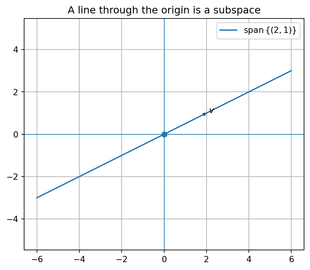
A line through the origin in \(\mathbb{R}^2\) or \(\mathbb{R}^3\) is a subspace.

For example,

\[ L=\left\{ t\begin{bmatrix}2\\1\end{bmatrix}:t\in\mathbb{R} \right\} \]

is a subspace of \(\mathbb{R}^2\).

It is the span of one vector:

\[ L=\operatorname{span} \left\{ \begin{bmatrix}2\\1\end{bmatrix} \right\}. \]

10.4.4 Planes through the origin

A plane through the origin in \(\mathbb{R}^3\) is a subspace.

For example,

\[ P= \operatorname{span} \left\{ \begin{bmatrix}1\\0\\1\end{bmatrix}, \begin{bmatrix}0\\1\\1\end{bmatrix} \right\} \]

is a plane through the origin.

10.5 8.3 Sets that are not subspaces

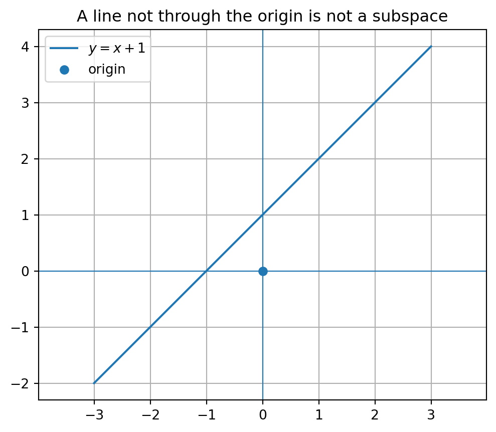
A line not passing through the origin is not a subspace.

For example,

\[ L=\left\{ \begin{bmatrix}x\\y\end{bmatrix}: y=x+1 \right\} \]

is not a subspace of \(\mathbb{R}^2\).

Why?

The zero vector is

\[ \begin{bmatrix}0\\0\end{bmatrix}. \]

But it does not satisfy \(y=x+1\), because

\[ 0\ne 0+1. \]

So \(0\notin L\).

Therefore \(L\) is not a subspace.

Similarly, a plane in \(\mathbb{R}^3\) not passing through the origin is not a subspace.

Origin test

If a subset of \(\mathbb{R}^n\) does not contain the zero vector, then it cannot be a subspace.

10.6 8.4 The subspace test

To prove a set is a subspace, use the definition.

Subspace test

A subset \(W\) of \(\mathbb{R}^n\) is a subspace if and only if:

\(0\in W\).
For all \(u,v\in W\), \(u+v\in W\).
For all \(u\in W\) and all \(c\in\mathbb{R}\), \(cu\in W\).

Sometimes conditions 2 and 3 are combined into one condition:

\[ u,v\in W,\ c,d\in\mathbb{R} \quad\Longrightarrow\quad cu+dv\in W. \]

This combined condition says that \(W\) is closed under all linear combinations.

10.7 8.5 Example: a subspace defined by an equation

Let

\[ W=\left\{ \begin{bmatrix}x\\y\\z\end{bmatrix} \in\mathbb{R}^3: x+2y-z=0 \right\}. \]

We show that \(W\) is a subspace.

First, the zero vector satisfies the equation:

\[ 0+2(0)-0=0. \]

So \(0\in W\).

Now let

\[ u= \begin{bmatrix}x_1\\y_1\\z_1\end{bmatrix}, \qquad v= \begin{bmatrix}x_2\\y_2\\z_2\end{bmatrix} \]

belong to \(W\). Then

\[ x_1+2y_1-z_1=0 \]

and

\[ x_2+2y_2-z_2=0. \]

For \(u+v\),

\[ (x_1+x_2)+2(y_1+y_2)-(z_1+z_2) = (x_1+2y_1-z_1)+(x_2+2y_2-z_2) = 0+0=0. \]

So \(u+v\in W\).

For a scalar \(c\),

\[ c u = \begin{bmatrix} cx_1\\ cy_1\\ cz_1 \end{bmatrix}. \]

Then

\[ cx_1+2cy_1-cz_1 = c(x_1+2y_1-z_1) = c\cdot 0 = 0. \]

So \(cu\in W\).

Therefore \(W\) is a subspace of \(\mathbb{R}^3\).

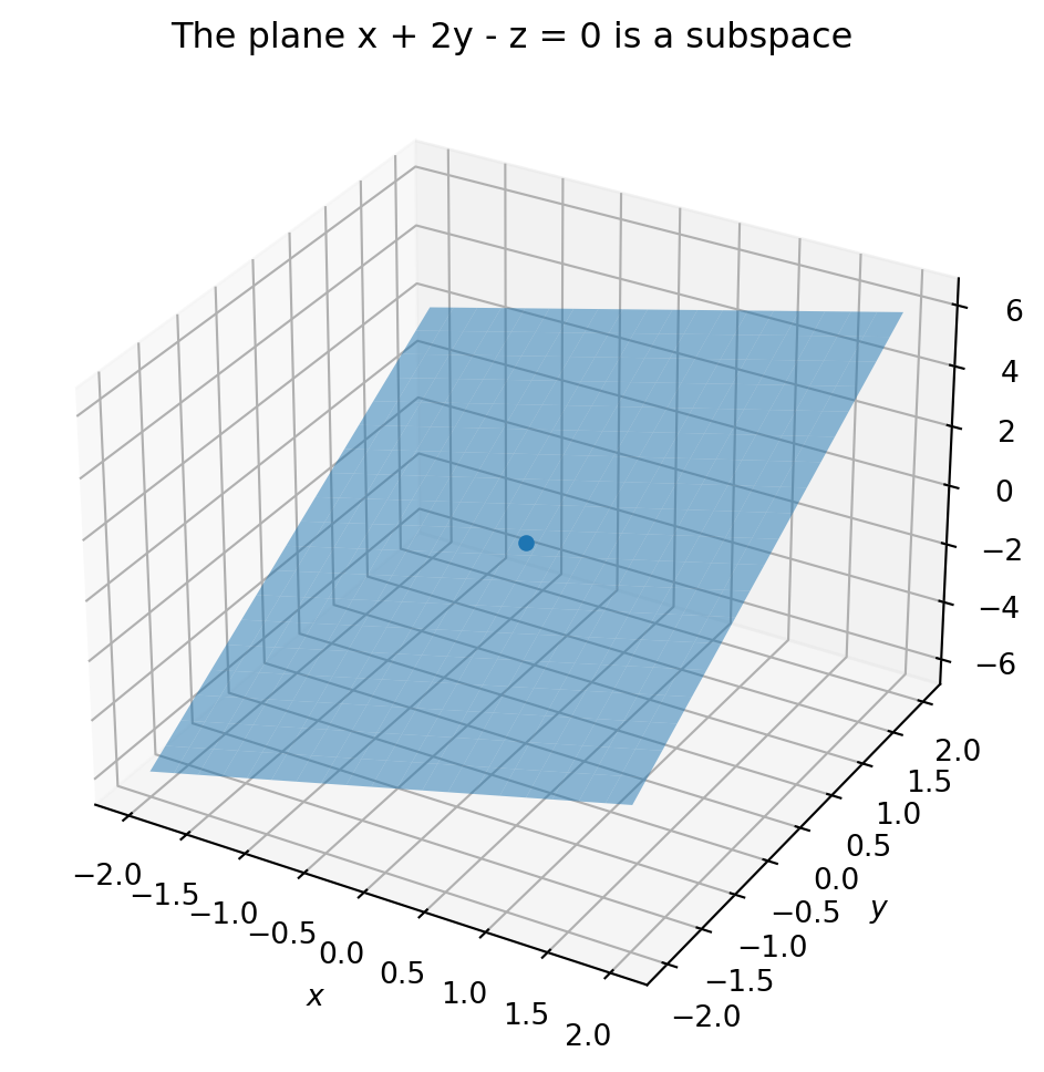
Geometrically, \(W\) is a plane through the origin.

10.8 8.6 Example: a set that fails closure

Let

\[ S=\left\{ \begin{bmatrix}x\\y\end{bmatrix}\in\mathbb{R}^2: xy=0 \right\}. \]

This set consists of points on the two coordinate axes.

It contains the zero vector, because \(0\cdot 0=0\).

It is closed under scalar multiplication: if \(xy=0\), then

\[ (cx)(cy)=c^2xy=0. \]

But it is not closed under addition.

The vector

\[ u= \begin{bmatrix}1\\0\end{bmatrix} \]

belongs to \(S\), and

\[ v= \begin{bmatrix}0\\1\end{bmatrix} \]

also belongs to \(S\).

But

\[ u+v= \begin{bmatrix}1\\1\end{bmatrix}, \]

and

\[ 1\cdot 1=1\ne 0. \]

So \(u+v\notin S\).

Therefore \(S\) is not a subspace.

This example shows that containing the zero vector is not enough. Both closure properties matter.

10.9 8.7 Every span is a subspace

Let

\[ W=\operatorname{span}\{v_1,v_2,\ldots,v_k\}. \]

Then \(W\) is a subspace.

Why?

The zero vector is in \(W\) because

\[ 0=0v_1+0v_2+\cdots+0v_k. \]

If \(u,v\in W\), then

\[ u=a_1v_1+\cdots+a_kv_k, \]

and

\[ v=b_1v_1+\cdots+b_kv_k. \]

Then

\[ u+v=(a_1+b_1)v_1+\cdots+(a_k+b_k)v_k, \]

which is still a linear combination of \(v_1,\ldots,v_k\). So \(u+v\in W\).

If \(c\in\mathbb{R}\), then

\[ cu=c(a_1v_1+\cdots+a_kv_k) = (ca_1)v_1+\cdots+(ca_k)v_k. \]

So \(cu\in W\).

Therefore every span is a subspace.

Span creates subspaces

The span of any set of vectors is always a subspace.

10.10 8.8 Homogeneous systems create subspaces

A homogeneous system has the form

\[ Ax=0. \]

The set of all solutions is a subspace of \(\mathbb{R}^n\).

Indeed, if \(u\) and \(v\) solve \(Ax=0\), then

\[ Au=0 \]

and

\[ Av=0. \]

Then

\[ A(u+v)=Au+Av=0+0=0. \]

So \(u+v\) is also a solution.

If \(c\) is a scalar, then

\[ A(cu)=cAu=c0=0. \]

So \(cu\) is also a solution.

Therefore the solution set of a homogeneous system is a subspace.

This subspace is called the nullspace of \(A\).

10.11 8.9 Nonhomogeneous systems usually do not create subspaces

A nonhomogeneous system has the form

\[ Ax=b, \]

where \(b\ne 0\).

Its solution set is usually not a subspace.

Why?

A subspace must contain the zero vector. But if \(b\ne 0\), then

\[ A0=0\ne b. \]

So \(0\) is not a solution.

Therefore the solution set of \(Ax=b\) is not a subspace when \(b\ne 0\).

It may be a shifted subspace, also called an affine subspace. For example, a line not through the origin is not a subspace, but it is a shifted copy of a one-dimensional subspace.

10.12 8.10 Column space

Definition: column space

The column space of a matrix \(A\) is the span of the columns of \(A\).

It is denoted

\[ \operatorname{Col}(A). \]

\[ A= \begin{bmatrix} |&|&&|\\ a_1&a_2&\cdots&a_n\\ |&|&&| \end{bmatrix}, \]

then

\[ \operatorname{Col}(A)=\operatorname{span}\{a_1,a_2,\ldots,a_n\}. \]

If \(A\) is an \(m\times n\) matrix, then each column is in \(\mathbb{R}^m\). Therefore

\[ \operatorname{Col}(A) \]

is a subspace of \(\mathbb{R}^m\).

The equation

\[ Ax=b \]

is consistent if and only if

\[ b\in\operatorname{Col}(A). \]

So the column space is the set of all possible outputs of the matrix transformation

\[ x\mapsto Ax. \]

10.13 8.11 Nullspace

Definition: nullspace

The nullspace of a matrix \(A\) is the set of all solutions to

\[ Ax=0. \]

It is denoted

\[ \operatorname{Null}(A). \]

If \(A\) is an \(m\times n\) matrix, then the equation \(Ax=0\) uses input vectors \(x\in\mathbb{R}^n\). Therefore

\[ \operatorname{Null}(A) \]

is a subspace of \(\mathbb{R}^n\).

The nullspace is the set of all inputs that are sent to zero.

Geometrically, it measures directions that the matrix cannot see.

Computationally, it measures degrees of freedom in the homogeneous system.

10.14 8.12 Row space

Definition: row space

The row space of a matrix \(A\) is the span of the rows of \(A\).

It is denoted

\[ \operatorname{Row}(A). \]

If \(A\) is an \(m\times n\) matrix, then each row has \(n\) entries. Therefore the row space is a subspace of \(\mathbb{R}^n\).

The row space is closely connected to the equations in a linear system.

Row reduction preserves the row space, because elementary row operations replace rows by linear combinations of rows and can be reversed.

Therefore, the nonzero rows of a row-echelon form of \(A\) form a basis for the row space.

10.15 8.13 The four fundamental subspaces preview

For an \(m\times n\) matrix \(A\), there are four important subspaces:

Subspace	Notation	Ambient space	Meaning
Column space	\(\operatorname{Col}(A)\)	\(\mathbb{R}^m\)	possible outputs \(Ax\)
Nullspace	\(\operatorname{Null}(A)\)	\(\mathbb{R}^n\)	inputs sent to \(0\)
Row space	\(\operatorname{Row}(A)\)	\(\mathbb{R}^n\)	span of equations
Left nullspace	\(\operatorname{Null}(A^T)\)	\(\mathbb{R}^m\)	constraints on outputs

We will return to all four subspaces when studying orthogonality and the fundamental theorem of linear algebra.

For now, we focus on the first three.

10.16 8.14 Finding a basis for the column space

To find a basis for \(\operatorname{Col}(A)\):

Row reduce \(A\).
Identify the pivot columns.
Select the corresponding columns from the original matrix \(A\).

Example:

\[ A= \begin{bmatrix} 1&2&0&3\\ 0&1&1&1\\ 1&3&1&4 \end{bmatrix}. \]

Row reduction gives

\[ \operatorname{rref}(A)= \begin{bmatrix} 1&0&-2&1\\ 0&1&1&1\\ 0&0&0&0 \end{bmatrix}. \]

The pivot columns are columns \(1\) and \(2\).

Therefore a basis for \(\operatorname{Col}(A)\) is given by the original columns

\[ \left\{ \begin{bmatrix} 1\\ 0\\ 1 \end{bmatrix}, \begin{bmatrix} 2\\ 1\\ 3 \end{bmatrix} \right\}. \]

Thus

\[ \dim(\operatorname{Col}(A))=2. \]

10.17 8.15 Finding a basis for the nullspace

To find a basis for \(\operatorname{Null}(A)\), solve

\[ Ax=0 \]

in parametric vector form.

Example:

\[ A= \begin{bmatrix} 1&2&0&3\\ 0&1&1&1\\ 1&3&1&4 \end{bmatrix}. \]

The rref is

\[ \begin{bmatrix} 1&0&-2&1\\ 0&1&1&1\\ 0&0&0&0 \end{bmatrix}. \]

The equations are

\[ x_1-2x_3+x_4=0, \]

\[ x_2+x_3+x_4=0. \]

The pivot variables are \(x_1\) and \(x_2\).

The free variables are \(x_3\) and \(x_4\).

Let

\[ x_3=s,\qquad x_4=t. \]

Then

\[ x_1=2s-t, \]

and

\[ x_2=-s-t. \]

Therefore

\[ x= \begin{bmatrix} x_1\\ x_2\\ x_3\\ x_4 \end{bmatrix} = \begin{bmatrix} 2s-t\\ -s-t\\ s\\ t \end{bmatrix} = s \begin{bmatrix} 2\\ -1\\ 1\\ 0 \end{bmatrix} + t \begin{bmatrix} -1\\ -1\\ 0\\ 1 \end{bmatrix}. \]

Thus a basis for \(\operatorname{Null}(A)\) is

\[ \left\{ \begin{bmatrix} 2\\ -1\\ 1\\ 0 \end{bmatrix}, \begin{bmatrix} -1\\ -1\\ 0\\ 1 \end{bmatrix} \right\}. \]

\[ \dim(\operatorname{Null}(A))=2. \]

10.18 8.16 Rank and nullity

The dimension of the column space is called the rank of \(A\).

The dimension of the nullspace is called the nullity of \(A\).

Definition: rank and nullity

For an \(m\times n\) matrix \(A\),

\[ \operatorname{rank}(A)=\dim(\operatorname{Col}(A)), \]

and

\[ \operatorname{nullity}(A)=\dim(\operatorname{Null}(A)). \]

The number of pivots is the rank.

The number of free variables is the nullity.

Since there are \(n\) variables total,

\[ \operatorname{rank}(A)+\operatorname{nullity}(A)=n. \]

This is the rank-nullity theorem.

Rank-nullity theorem

If \(A\) is an \(m\times n\) matrix, then

\[ \operatorname{rank}(A)+\operatorname{nullity}(A)=n. \]

10.19 8.17 Geometry of rank and nullity

Rank counts independent output directions.

Nullity counts invisible input directions.

For a matrix

\[ A:\mathbb{R}^n\to\mathbb{R}^m, \]

the input space has dimension \(n\).

Some directions are visible in the output. These form the rank.

Some directions collapse to zero. These form the nullity.

Rank-nullity says:

\[ \text{input dimension} = \text{visible dimension} + \text{invisible dimension}. \]

That is,

\[ n=\operatorname{rank}(A)+\operatorname{nullity}(A). \]

10.20 8.18 Python: visualizing subspaces in \(\mathbb{R}^2\)

A line through the origin is a subspace of \(\mathbb{R}^2\).

import numpy as np
import matplotlib.pyplot as plt

v = np.array([2, 1], dtype=float)
t = np.linspace(-3, 3, 200)
line = np.outer(t, v)

plt.figure(figsize=(6, 5))
plt.plot(line[:, 0], line[:, 1], label=r"$\operatorname{span}\{(2,1)\}$")
plt.arrow(0, 0, v[0], v[1], head_width=0.1, length_includes_head=True)
plt.text(v[0] + 0.1, v[1], "$v$")
plt.scatter([0], [0])
plt.axhline(0, linewidth=0.8)
plt.axvline(0, linewidth=0.8)
plt.grid(True)
plt.axis("equal")
plt.title("A line through the origin is a subspace")
plt.legend()
plt.show()

A line not through the origin is not a subspace.

x = np.linspace(-3, 3, 200)
y = x + 1

plt.figure(figsize=(6, 5))
plt.plot(x, y, label="$y=x+1$")
plt.scatter([0], [0], label="origin")
plt.axhline(0, linewidth=0.8)
plt.axvline(0, linewidth=0.8)
plt.grid(True)
plt.axis("equal")
plt.title("A line not through the origin is not a subspace")
plt.legend()
plt.show()

10.21 8.19 Python: visualizing a plane subspace in \(\mathbb{R}^3\)

The equation

\[ x+2y-z=0 \]

defines a plane through the origin, hence a subspace.

Solve for \(z\):

\[ z=x+2y. \]

from mpl_toolkits.mplot3d import Axes3D

x = np.linspace(-2, 2, 20)
y = np.linspace(-2, 2, 20)
X, Y = np.meshgrid(x, y)
Z = X + 2*Y

fig = plt.figure(figsize=(7, 6))
ax = fig.add_subplot(111, projection="3d")
ax.plot_surface(X, Y, Z, alpha=0.5)
ax.scatter([0], [0], [0])
ax.set_xlabel("$x$")
ax.set_ylabel("$y$")
ax.set_zlabel("$z$")
ax.set_title("The plane x + 2y - z = 0 is a subspace")
plt.show()

The equation

\[ x+2y-z=1 \]

defines a parallel plane not passing through the origin. It is not a subspace.

10.22 8.20 Python: column space and nullspace with SymPy

import sympy as sp

A = sp.Matrix([
    [1, 2, 0, 3],
    [0, 1, 1, 1],
    [1, 3, 1, 4]
])

rref_A, pivots = A.rref()
rref_A, pivots

(Matrix([
 [1, 0, -2, 1],
 [0, 1,  1, 1],
 [0, 0,  0, 0]]),
 (0, 1))

The pivot columns identify a basis for the column space.

col_basis = [A[:, j] for j in pivots]
col_basis

[Matrix([
 [1],
 [0],
 [1]]),
 Matrix([
 [2],
 [1],
 [3]])]

SymPy can also compute a nullspace basis directly.

null_basis = A.nullspace()
null_basis

[Matrix([
 [ 2],
 [-1],
 [ 1],
 [ 0]]),
 Matrix([
 [-1],
 [-1],
 [ 0],
 [ 1]])]

The vectors in null_basis form a basis for \(\operatorname{Null}(A)\).

10.23 8.21 Python: checking rank-nullity

rank = A.rank()
nullity = len(A.nullspace())
n = A.shape[1]

rank, nullity, n, rank + nullity

(2, 2, 4, 4)

The result should satisfy

\[ \operatorname{rank}(A)+\operatorname{nullity}(A)=n. \]

10.24 8.22 Algorithmic summary

Algorithm: test whether a set is a subspace

To test whether \(W\subseteq\mathbb{R}^n\) is a subspace:

Check whether \(0\in W\).
Check closure under addition.
Check closure under scalar multiplication.

If all three conditions hold, \(W\) is a subspace.

Algorithm: find a basis for \(\operatorname{Col}(A)\)

Row reduce \(A\).
Identify the pivot column positions.
Select the corresponding columns from the original matrix \(A\).
These original pivot columns form a basis for \(\operatorname{Col}(A)\).

Algorithm: find a basis for \(\operatorname{Null}(A)\)

Solve \(Ax=0\).
Write the solution in parametric vector form.
The direction vectors attached to free parameters form a basis for \(\operatorname{Null}(A)\).

10.25 8.23 Common mistakes

10.25.1 Mistake 1: forgetting the zero vector condition

If a set does not contain \(0\), it is not a subspace.

10.25.2 Mistake 2: thinking every line is a subspace

Only lines through the origin are subspaces.

10.25.3 Mistake 3: thinking every plane is a subspace

Only planes through the origin are subspaces.

10.25.4 Mistake 4: using nonhomogeneous solution sets as subspaces

The solution set of \(Ax=b\) is not a subspace when \(b\ne 0\).

10.25.5 Mistake 5: using rref columns as a basis for the column space

Use pivot columns from the original matrix, not the rref matrix.

10.25.6 Mistake 6: confusing column space and nullspace

For an \(m\times n\) matrix:

\[ \operatorname{Col}(A)\subseteq\mathbb{R}^m, \]

but

\[ \operatorname{Null}(A)\subseteq\mathbb{R}^n. \]

They usually live in different spaces.

10.26 8.24 Chapter summary

A subspace of \(\mathbb{R}^n\) is a subset that contains \(0\) and is closed under addition and scalar multiplication.

Every span is a subspace.

The solution set of a homogeneous system \(Ax=0\) is a subspace.

The solution set of a nonhomogeneous system \(Ax=b\) is usually not a subspace.

The column space of \(A\) is the span of its columns:

\[ \operatorname{Col}(A)=\operatorname{span}\{\text{columns of }A\}. \]

The nullspace of \(A\) is the solution set of

\[ Ax=0. \]

The row space of \(A\) is the span of its rows.

The rank of \(A\) is

\[ \operatorname{rank}(A)=\dim(\operatorname{Col}(A)). \]

The nullity of \(A\) is

\[ \operatorname{nullity}(A)=\dim(\operatorname{Null}(A)). \]

The rank-nullity theorem says

\[ \operatorname{rank}(A)+\operatorname{nullity}(A)=n \]

for an \(m\times n\) matrix.

10.27 Exercises

10.27.1 A. Subspace test

Determine whether each set is a subspace of the indicated space. Justify your answer.

\[ W=\left\{ \begin{bmatrix}x\\y\end{bmatrix}\in\mathbb{R}^2: y=2x \right\}. \]

\[ W=\left\{ \begin{bmatrix}x\\y\end{bmatrix}\in\mathbb{R}^2: y=2x+1 \right\}. \]

\[ W=\left\{ \begin{bmatrix}x\\y\\z\end{bmatrix}\in\mathbb{R}^3: x+2y-z=0 \right\}. \]

\[ W=\left\{ \begin{bmatrix}x\\y\\z\end{bmatrix}\in\mathbb{R}^3: x+2y-z=1 \right\}. \]

\[ W=\left\{ \begin{bmatrix}x\\y\end{bmatrix}\in\mathbb{R}^2: xy=0 \right\}. \]

10.27.2 B. Spans as subspaces

For each set, describe the span geometrically and give its dimension.

\[ \operatorname{span} \left\{ \begin{bmatrix}2\\1\end{bmatrix} \right\} \]

\[ \operatorname{span} \left\{ \begin{bmatrix}1\\2\end{bmatrix}, \begin{bmatrix}2\\4\end{bmatrix} \right\} \]

\[ \operatorname{span} \left\{ \begin{bmatrix}1\\2\end{bmatrix}, \begin{bmatrix}1\\-1\end{bmatrix} \right\} \]

\[ \operatorname{span} \left\{ \begin{bmatrix}1\\0\\1\end{bmatrix}, \begin{bmatrix}0\\1\\1\end{bmatrix} \right\} \]

10.27.3 C. Column space

Find a basis for the column space of each matrix and give its rank.

\[ A= \begin{bmatrix} 1&2&0&3\\ 0&1&1&1\\ 1&3&1&4 \end{bmatrix} \]

\[ B= \begin{bmatrix} 1&2&3\\ 2&4&6\\ 1&1&1 \end{bmatrix} \]

\[ C= \begin{bmatrix} 1&0&2&1\\ 0&1&3&-1\\ 0&0&0&0 \end{bmatrix} \]

10.27.4 D. Nullspace

Find a basis for the nullspace of each matrix and give its nullity.

\[ A= \begin{bmatrix} 1&2&0&3\\ 0&1&1&1\\ 1&3&1&4 \end{bmatrix} \]

\[ B= \begin{bmatrix} 1&2&3\\ 2&4&6\\ 1&1&1 \end{bmatrix} \]

\[ C= \begin{bmatrix} 1&0&2&1\\ 0&1&3&-1\\ 0&0&0&0 \end{bmatrix} \]

10.27.5 E. Rank-nullity

For each matrix, find rank, nullity, and verify rank-nullity.

A \(3\times 5\) matrix with \(3\) pivots.
A \(4\times 4\) matrix with \(4\) pivots.
A \(5\times 3\) matrix with \(2\) pivots.
A \(2\times 6\) matrix with \(2\) pivots.

10.27.6 F. Conceptual questions

Why is every span a subspace?
Why is the solution set of \(Ax=0\) a subspace?
Why is the solution set of \(Ax=b\) usually not a subspace when \(b\ne 0\)?
What is the difference between column space and nullspace?
What does rank measure?
What does nullity measure?

10.27.7 G. Python exercises

Plot the line

\[ \operatorname{span} \left\{ \begin{bmatrix}2\\1\end{bmatrix} \right\}. \]

Plot the line \(y=x+1\) and explain why it is not a subspace.
Use SymPy to find the rref, pivot columns, column-space basis, and nullspace basis for

\[ A= \begin{bmatrix} 1&2&0&3\\ 0&1&1&1\\ 1&3&1&4 \end{bmatrix}. \]

Verify rank-nullity for the matrix in part 3.
Create a \(3\)D plot of the plane

\[ x+2y-z=0. \]

10.27.8 H. Reflection

Write a short paragraph answering each question.

Why are subspaces the natural setting for linear algebra?
How does a column space describe possible outputs?
How does a nullspace describe invisible inputs?
Why is rank-nullity a conservation law for dimension?
How do subspaces help organize data and computation?

10.28 AI-age connection

Subspaces are essential in data science and AI because high-dimensional data often lives near lower-dimensional structure. A collection of images, signals, or feature vectors may appear to occupy a huge ambient space, but much of its meaningful variation may lie in a smaller subspace or near a low-dimensional manifold. Column spaces describe what a model can produce. Nullspaces describe what a model cannot detect. Rank and nullity measure visible and invisible dimensions. These ideas prepare the way for least squares, projections, PCA, and the SVD.