4 Matrices, Vectors, and Augmented Systems

4.1 Opening question

In Chapter 1, we solved systems of equations by writing and rewriting equations.

But equations can become long. If a system has many variables and many equations, the symbols \(x_1,x_2,\ldots,x_n\) take up space, and the actual computation depends mostly on the coefficients.

For example, the system

\[ \begin{cases} x_1-3x_2-5x_3=1,\\ x_1-x_2-2x_3=0,\\ 3x_1-x_2+x_3=3 \end{cases} \]

is completely determined by the rectangular array

\[ \left[ \begin{array}{ccc|c} 1&-3&-5&1\\ 1&-1&-2&0\\ 3&-1&1&3 \end{array} \right]. \]

This chapter introduces the objects that make this possible:

matrices,
vectors,
augmented matrices,
matrix-vector multiplication,
and the compact equation \(Ax=b\).

The key idea is:

A matrix stores a linear system, and matrix-vector multiplication turns a system into one equation.

4.2 Learning goals

After studying this chapter, you should be able to:

Identify the size of a matrix.
Use row-column notation for matrix entries.
Distinguish matrices, column vectors, and row vectors.
Understand vectors as objects in \(\mathbb{R}^n\).
Form coefficient matrices and augmented matrices from linear systems.
Add matrices and multiply matrices by scalars.
Compute matrix-vector products.
Interpret \(Ax\) as a linear combination of the columns of \(A\).
Write a linear system in the compact form \(Ax=b\).
Use Python to create and compute with matrices and vectors.

4.3 2.1 Matrices as rectangular arrays

Definition: matrix

An \(m\times n\) matrix is a rectangular array of numbers with \(m\) rows and \(n\) columns.

For example,

\[ A= \begin{bmatrix} 1&-3&-5\\ 1&-1&-2\\ 3&-1&1 \end{bmatrix} \]

is a \(3\times 3\) matrix.

The matrix

\[ B= \begin{bmatrix} 2&0&1&5\\ -1&3&4&2 \end{bmatrix} \]

is a \(2\times 4\) matrix.

The size is always written as

\[ \text{number of rows}\times \text{number of columns}. \]

So a \(2\times 4\) matrix has \(2\) rows and \(4\) columns.

4.4 2.2 Matrix entries

If \(A\) is a matrix, then \(a_{ij}\) denotes the entry in row \(i\) and column \(j\).

For example, if

\[ A= \begin{bmatrix} 4&-1&0\\ 2&5&7 \end{bmatrix}, \]

then

\[ a_{11}=4,\qquad a_{12}=-1,\qquad a_{23}=7. \]

The first subscript tells the row. The second subscript tells the column.

Memory rule

The entry \(a_{ij}\) is in row \(i\), column \(j\).

Row comes first. Column comes second.

4.5 2.3 Special matrices

4.5.1 Square matrices

A matrix is square if it has the same number of rows and columns.

For example,

\[ \begin{bmatrix} 1&2\\ 3&4 \end{bmatrix} \]

is a \(2\times 2\) square matrix, and

\[ \begin{bmatrix} 1&0&2\\ -1&3&5\\ 4&2&1 \end{bmatrix} \]

is a \(3\times 3\) square matrix.

4.5.2 The main diagonal

In a square matrix, the entries

\[ a_{11},a_{22},\ldots,a_{nn} \]

form the main diagonal.

For example, in

\[ A= \begin{bmatrix} 2&5&1\\ 0&-3&4\\ 7&8&6 \end{bmatrix}, \]

the diagonal entries are

\[ 2,\quad -3,\quad 6. \]

4.5.3 Diagonal matrices

A square matrix is diagonal if all entries off the main diagonal are zero.

Example:

\[ D= \begin{bmatrix} 2&0&0\\ 0&-3&0\\ 0&0&6 \end{bmatrix}. \]

4.5.4 Zero matrices

A zero matrix is a matrix whose entries are all zero.

For example,

\[ 0_{2\times 3}= \begin{bmatrix} 0&0&0\\ 0&0&0 \end{bmatrix}. \]

Usually we simply write \(0\) when the size is clear from context.

4.5.5 Identity matrices

The \(n\times n\) identity matrix is

\[ I_n= \begin{bmatrix} 1&0&\cdots&0\\ 0&1&\cdots&0\\ \vdots&\vdots&\ddots&\vdots\\ 0&0&\cdots&1 \end{bmatrix}. \]

For example,

\[ I_3= \begin{bmatrix} 1&0&0\\ 0&1&0\\ 0&0&1 \end{bmatrix}. \]

The identity matrix plays the same role for matrices that the number \(1\) plays for ordinary multiplication.

4.6 2.4 Vectors in \(\mathbb{R}^n\)

Definition: vector in \(\mathbb{R}^n\)

A vector in \(\mathbb{R}^n\) is an ordered list of \(n\) real numbers.

In this book, vectors are usually written as column vectors:

\[ v= \begin{bmatrix} v_1\\ v_2\\ \vdots\\ v_n \end{bmatrix}. \]

For example,

\[ v= \begin{bmatrix} 2\\ -1\\ 5 \end{bmatrix} \]

is a vector in \(\mathbb{R}^3\).

The entries of a vector are called its components.

A vector may represent many different kinds of data:

a point in space,
a displacement,
a velocity,
a list of measurements,
a pixel intensity vector,
a feature vector in machine learning,
a probability distribution,
a signal,
a document embedding.

In computational linear algebra, a vector is both a geometric object and a data object.

4.7 2.5 Column vectors and row vectors

A matrix with only one column is a column vector.

Example:

\[ \begin{bmatrix} 1\\ 4\\ -2 \end{bmatrix}. \]

A matrix with only one row is a row vector.

Example:

\[ \begin{bmatrix} 1&4&-2 \end{bmatrix}. \]

In this book, unless otherwise stated, the word vector means column vector.

The reason is that matrix-vector multiplication is naturally written as

\[ Ax, \]

where \(x\) is a column vector.

4.8 2.6 Geometric representation of vectors

A vector in \(\mathbb{R}^2\),

\[ v= \begin{bmatrix} a\\ b \end{bmatrix}, \]

can be drawn as an arrow from the origin to the point \((a,b)\).

For example,

\[ v= \begin{bmatrix} 3\\ 2 \end{bmatrix} \]

is drawn as an arrow from \((0,0)\) to \((3,2)\).

A vector in \(\mathbb{R}^3\),

\[ v= \begin{bmatrix} a\\ b\\ c \end{bmatrix}, \]

is drawn as an arrow from the origin to the point \((a,b,c)\).

In higher dimensions, we cannot draw the vector directly, but the same idea remains:

\[ \begin{bmatrix} v_1\\ v_2\\ \vdots\\ v_n \end{bmatrix} \]

is an object with \(n\) components.

4.9 2.7 Matrix addition

Matrices of the same size can be added component by component.

\[ A= \begin{bmatrix} 1&2&0\\ -1&3&4 \end{bmatrix}, \qquad B= \begin{bmatrix} 5&-2&1\\ 0&7&-3 \end{bmatrix}, \]

then

\[ A+B= \begin{bmatrix} 1+5&2+(-2)&0+1\\ -1+0&3+7&4+(-3) \end{bmatrix} = \begin{bmatrix} 6&0&1\\ -1&10&1 \end{bmatrix}. \]

Matrix addition is only defined when the matrices have the same size.

4.10 2.8 Scalar multiplication

A real number is often called a scalar.

To multiply a matrix by a scalar, multiply every entry by that scalar.

\[ A= \begin{bmatrix} 1&-2&0\\ 3&4&-1 \end{bmatrix}, \]

then

\[ -3A= \begin{bmatrix} -3&6&0\\ -9&-12&3 \end{bmatrix}. \]

The same rule applies to vectors:

\[ 2 \begin{bmatrix} 1\\ -3\\ 4 \end{bmatrix} = \begin{bmatrix} 2\\ -6\\ 8 \end{bmatrix}. \]

4.11 2.9 Basic algebraic rules

For matrices \(A,B,C\) of the same size and scalars \(c,d\), we have:

\[ A+B=B+A, \]

\[ (A+B)+C=A+(B+C), \]

\[ c(A+B)=cA+cB, \]

\[ (c+d)A=cA+dA, \]

\[ c(dA)=(cd)A. \]

These rules look familiar because matrix addition and scalar multiplication are defined entry by entry.

4.12 2.10 Transpose

Definition: transpose

The transpose of a matrix \(A\), written \(A^T\), is obtained by turning rows into columns and columns into rows.

For example,

\[ A= \begin{bmatrix} 2&-1&0\\ -2&5&1 \end{bmatrix} \]

has transpose

\[ A^T= \begin{bmatrix} 2&-2\\ -1&5\\ 0&1 \end{bmatrix}. \]

If \(A\) is \(m\times n\), then \(A^T\) is \(n\times m\).

A column vector transposes into a row vector:

\[ v= \begin{bmatrix} v_1\\ v_2\\ v_3 \end{bmatrix}, \qquad v^T= \begin{bmatrix} v_1&v_2&v_3 \end{bmatrix}. \]

A matrix \(A\) is symmetric if

\[ A^T=A. \]

For example,

\[ \begin{bmatrix} 2&3\\ 3&-1 \end{bmatrix} \]

is symmetric.

4.13 2.11 From linear systems to matrices

Consider the system

\[ \begin{cases} 2x+8y+4z=2,\\ 2x+5y+z=5,\\ 4x+10y-z=1. \end{cases} \]

The coefficient matrix is

\[ A= \begin{bmatrix} 2&8&4\\ 2&5&1\\ 4&10&-1 \end{bmatrix}. \]

The right-hand side vector is

\[ b= \begin{bmatrix} 2\\ 5\\ 1 \end{bmatrix}. \]

The vector of unknowns is

\[ x= \begin{bmatrix} x\\ y\\ z \end{bmatrix}. \]

The system can be written compactly as

\[ Ax=b. \]

The augmented matrix is

\[ \left[ \begin{array}{ccc|c} 2&8&4&2\\ 2&5&1&5\\ 4&10&-1&1 \end{array} \right]. \]

The vertical line is not part of the matrix algebra. It is a visual reminder of where the equals signs were in the original system.

4.14 2.12 The compact equation \(Ax=b\)

The notation

\[ Ax=b \]

is one of the most important expressions in all of linear algebra.

It represents the system

\[ \begin{cases} a_{11}x_1+a_{12}x_2+\cdots+a_{1n}x_n=b_1,\\ a_{21}x_1+a_{22}x_2+\cdots+a_{2n}x_n=b_2,\\ \vdots\\ a_{m1}x_1+a_{m2}x_2+\cdots+a_{mn}x_n=b_m. \end{cases} \]

Here

\[ A= \begin{bmatrix} a_{11}&a_{12}&\cdots&a_{1n}\\ a_{21}&a_{22}&\cdots&a_{2n}\\ \vdots&\vdots&\ddots&\vdots\\ a_{m1}&a_{m2}&\cdots&a_{mn} \end{bmatrix}, \]

\[ x= \begin{bmatrix} x_1\\ x_2\\ \vdots\\ x_n \end{bmatrix}, \qquad b= \begin{bmatrix} b_1\\ b_2\\ \vdots\\ b_m \end{bmatrix}. \]

The matrix \(A\) has size \(m\times n\), the unknown vector \(x\) has size \(n\times 1\), and the right-hand side vector \(b\) has size \(m\times 1\).

4.15 2.13 Matrix-vector multiplication

Let

\[ A= \begin{bmatrix} a_{11}&a_{12}&\cdots&a_{1n}\\ a_{21}&a_{22}&\cdots&a_{2n}\\ \vdots&\vdots&\ddots&\vdots\\ a_{m1}&a_{m2}&\cdots&a_{mn} \end{bmatrix} \]

and

\[ x= \begin{bmatrix} x_1\\ x_2\\ \vdots\\ x_n \end{bmatrix}. \]

Then \(Ax\) is the vector

\[ Ax= \begin{bmatrix} a_{11}x_1+a_{12}x_2+\cdots+a_{1n}x_n\\ a_{21}x_1+a_{22}x_2+\cdots+a_{2n}x_n\\ \vdots\\ a_{m1}x_1+a_{m2}x_2+\cdots+a_{mn}x_n \end{bmatrix}. \]

Each component of \(Ax\) is a dot product between a row of \(A\) and the vector \(x\).

4.15.1 Example

Let

\[ A= \begin{bmatrix} 1&2&3\\ 4&5&6 \end{bmatrix}, \qquad x= \begin{bmatrix} 2\\ -1\\ 3 \end{bmatrix}. \]

Then

\[ Ax= \begin{bmatrix} 1(2)+2(-1)+3(3)\\ 4(2)+5(-1)+6(3) \end{bmatrix} = \begin{bmatrix} 9\\ 21 \end{bmatrix}. \]

4.16 2.14 Dimension compatibility

Matrix-vector multiplication \(Ax\) is defined only when the number of columns of \(A\) equals the number of entries of \(x\).

If \(A\) is \(m\times n\), then \(x\) must be in \(\mathbb{R}^n\), and \(Ax\) will be in \(\mathbb{R}^m\):

\[ \underbrace{A}_{m\times n} \underbrace{x}_{n\times 1} = \underbrace{Ax}_{m\times 1}. \]

Example:

\[ \begin{bmatrix} 1&2&3\\ 4&5&6 \end{bmatrix} \begin{bmatrix} 1\\ 0\\ -1 \end{bmatrix} \]

is defined because a \(2\times 3\) matrix can multiply a \(3\times 1\) vector.

But

\[ \begin{bmatrix} 1&2&3\\ 4&5&6 \end{bmatrix} \begin{bmatrix} 1\\ 0 \end{bmatrix} \]

is not defined, because the dimensions do not match.

4.17 2.15 The column-combination view

Matrix-vector multiplication has another interpretation that is even more important.

Let the columns of \(A\) be

\[ A= \begin{bmatrix} |&|&&|\\ a_1&a_2&\cdots&a_n\\ |&|&&| \end{bmatrix}. \]

Then

\[ Ax= A \begin{bmatrix} x_1\\ x_2\\ \vdots\\ x_n \end{bmatrix} = x_1a_1+x_2a_2+\cdots+x_na_n. \]

So \(Ax\) is a linear combination of the columns of \(A\).

This is the column picture.

4.17.1 Example

Let

\[ A= \begin{bmatrix} 1&1\\ 2&-1 \end{bmatrix}, \qquad x= \begin{bmatrix} 2\\ 3 \end{bmatrix}. \]

Then

\[ Ax = 2 \begin{bmatrix} 1\\ 2 \end{bmatrix} + 3 \begin{bmatrix} 1\\ -1 \end{bmatrix} = \begin{bmatrix} 2\\ 4 \end{bmatrix} + \begin{bmatrix} 3\\ -3 \end{bmatrix} = \begin{bmatrix} 5\\ 1 \end{bmatrix}. \]

Thus the equation

\[ Ax=b \]

asks:

Can the vector \(b\) be written as a linear combination of the columns of \(A\)?

This question will lead us to span, column space, rank, and basis.

4.18 2.16 Row picture versus column picture

Consider

\[ \begin{bmatrix} 1&1\\ 2&-1 \end{bmatrix} \begin{bmatrix} x_1\\ x_2 \end{bmatrix} = \begin{bmatrix} 5\\ 1 \end{bmatrix}. \]

4.18.1 Row picture

The system is

\[ x_1+x_2=5, \]

\[ 2x_1-x_2=1. \]

Each equation is a line. The solution is the intersection of the two lines.

Solving gives

\[ (x_1,x_2)=(2,3). \]

4.18.2 Column picture

The same system can be written as

\[ x_1 \begin{bmatrix} 1\\ 2 \end{bmatrix} + x_2 \begin{bmatrix} 1\\ -1 \end{bmatrix} = \begin{bmatrix} 5\\ 1 \end{bmatrix}. \]

Using the solution \((x_1,x_2)=(2,3)\),

\[ 2 \begin{bmatrix} 1\\ 2 \end{bmatrix} + 3 \begin{bmatrix} 1\\ -1 \end{bmatrix} = \begin{bmatrix} 5\\ 1 \end{bmatrix}. \]

The row picture asks where equations intersect.

The column picture asks how to build \(b\) from the columns of \(A\).

Both pictures describe the same system.

4.19 2.17 Linear combinations

Definition: linear combination

A linear combination of vectors \(v_1,v_2,\ldots,v_k\) is a vector of the form

\[ c_1v_1+c_2v_2+\cdots+c_kv_k, \]

where \(c_1,c_2,\ldots,c_k\) are scalars.

Matrix-vector multiplication is a machine for producing linear combinations.

\[ A= \begin{bmatrix} |&|&&|\\ v_1&v_2&\cdots&v_k\\ |&|&&| \end{bmatrix}, \]

then

\[ Ax=c_1v_1+c_2v_2+\cdots+c_kv_k \]

where

\[ x= \begin{bmatrix} c_1\\ c_2\\ \vdots\\ c_k \end{bmatrix}. \]

This is why matrices are so important: they package many possible linear combinations into a single object.

4.20 2.18 Writing systems as augmented matrices

To write a system as an augmented matrix:

Choose an order for the variables.
Write the coefficients in that order.
Place the right-hand side in the last column.
Use a vertical bar to separate coefficients from constants.

Example:

\[ \begin{cases} x_2+3x_3=7,\\ x_1+3x_2+2x_3=-3,\\ 2x_1+5x_2+x_3=-1. \end{cases} \]

Using variable order \(x_1,x_2,x_3\), the augmented matrix is

\[ \left[ \begin{array}{ccc|c} 0&1&3&7\\ 1&3&2&-3\\ 2&5&1&-1 \end{array} \right]. \]

Notice the zero in the first row, first column, because the first equation has no \(x_1\) term.

Common mistake

Do not change the variable order from row to row.

If the variable order is \(x_1,x_2,x_3\), every row must follow that order.

4.21 2.19 Data interpretation

Vectors and matrices are not only algebraic objects. They are also data structures.

A vector may store one observation:

\[ v= \begin{bmatrix} \text{height}\\ \text{weight}\\ \text{age}\\ \text{income} \end{bmatrix}. \]

A matrix may store many observations:

\[ X= \begin{bmatrix} \text{--- person 1 ---}\\ \text{--- person 2 ---}\\ \vdots\\ \text{--- person m ---} \end{bmatrix}. \]

In data science, a common convention is:

rows are observations,
columns are features.

For example, a data matrix might be

\[ X= \begin{bmatrix} 65&120&20\\ 70&160&25\\ 68&140&22 \end{bmatrix}, \]

where the columns represent height, weight, and age.

Linear algebra gives us the language to transform, compare, compress, and model such data.

4.22 2.20 First Python computations with matrices

import numpy as np

A = np.array([
    [1, -3, -5],
    [1, -1, -2],
    [3, -1,  1]
], dtype=float)

b = np.array([1, 0, 3], dtype=float)

A

array([[ 1., -3., -5.],
       [ 1., -1., -2.],
       [ 3., -1.,  1.]])

array([1., 0., 3.])

4.22.1 Matrix shape

A.shape

(3, 3)

This tells us that \(A\) has \(3\) rows and \(3\) columns.

4.22.2 Accessing entries

Python uses zero-based indexing. So A[0,0] is the mathematical entry \(a_{11}\).

A[0, 0], A[1, 2]

(1.0, -2.0)

4.22.3 Matrix-vector multiplication

x = np.array([0, -2, 1], dtype=float)
A @ x

array([1., 0., 3.])

This returns \(b\), so \(x\) solves \(Ax=b\).

4.22.4 Transpose

A.T

array([[ 1.,  1.,  3.],
       [-3., -1., -1.],
       [-5., -2.,  1.]])

4.22.5 Matrix addition and scalar multiplication

2 * A

array([[  2.,  -6., -10.],
       [  2.,  -2.,  -4.],
       [  6.,  -2.,   2.]])

A + A

array([[  2.,  -6., -10.],
       [  2.,  -2.,  -4.],
       [  6.,  -2.,   2.]])

4.23 2.21 Visualizing matrix-vector multiplication

For a \(2\times 2\) matrix, matrix-vector multiplication transforms vectors in the plane.

Let

\[ A= \begin{bmatrix} 1&1\\ 2&-1 \end{bmatrix}. \]

Then

\[ A \begin{bmatrix} x\\ y \end{bmatrix} = x \begin{bmatrix} 1\\ 2 \end{bmatrix} + y \begin{bmatrix} 1\\ -1 \end{bmatrix}. \]

The standard basis vectors

\[ e_1= \begin{bmatrix} 1\\ 0 \end{bmatrix}, \qquad e_2= \begin{bmatrix} 0\\ 1 \end{bmatrix} \]

are sent to the columns of \(A\):

\[ Ae_1= \begin{bmatrix} 1\\ 2 \end{bmatrix}, \qquad Ae_2= \begin{bmatrix} 1\\ -1 \end{bmatrix}. \]

Thus the columns of \(A\) tell us where the coordinate axes go.

import matplotlib.pyplot as plt

A2 = np.array([[1, 1],
               [2, -1]], dtype=float)

e1 = np.array([1, 0])
e2 = np.array([0, 1])

Ae1 = A2 @ e1
Ae2 = A2 @ e2

plt.figure()
plt.arrow(0, 0, e1[0], e1[1], head_width=0.08, length_includes_head=True, label="$e_1$")
plt.arrow(0, 0, e2[0], e2[1], head_width=0.08, length_includes_head=True)
plt.arrow(0, 0, Ae1[0], Ae1[1], head_width=0.08, length_includes_head=True)
plt.arrow(0, 0, Ae2[0], Ae2[1], head_width=0.08, length_includes_head=True)
plt.text(e1[0]+0.05, e1[1], "$e_1$")
plt.text(e2[0], e2[1]+0.05, "$e_2$")
plt.text(Ae1[0]+0.05, Ae1[1], "$Ae_1$")
plt.text(Ae2[0]+0.05, Ae2[1], "$Ae_2$")
plt.axhline(0, linewidth=0.8)
plt.axvline(0, linewidth=0.8)
plt.grid(True)
plt.axis("equal")
plt.title("Columns of A are images of standard basis vectors")
plt.show()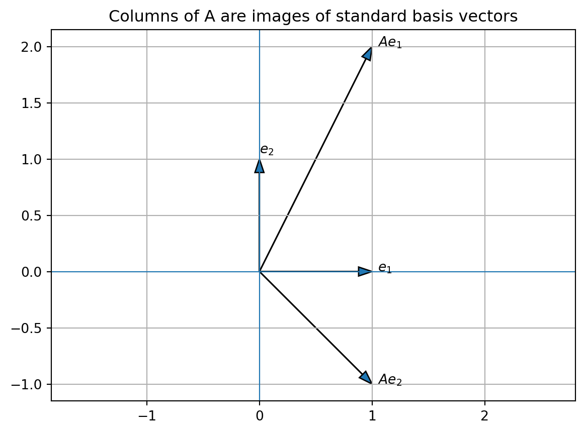

4.24 2.22 Algorithmic summary

Algorithm: convert a system to \(Ax=b\)

Given a linear system:

Choose an order for the variables.
Build \(A\) from the coefficients.
Build \(x\) as the column vector of variables.
Build \(b\) from the right-hand side constants.
Write the system as \(Ax=b\).
Build the augmented matrix \([A\mid b]\) when preparing for elimination.

4.25 2.23 Common mistakes

4.25.1 Mistake 1: confusing rows and columns

A \(3\times 4\) matrix has \(3\) rows and \(4\) columns, not the other way around.

4.25.2 Mistake 2: forgetting zero coefficients

The equation

\[ x_2+3x_3=7 \]

has coefficient \(0\) for \(x_1\). With variable order \(x_1,x_2,x_3\), the row is

\[ [0\quad 1\quad 3\mid 7]. \]

4.25.3 Mistake 3: multiplying dimensions incorrectly

If \(A\) is \(m\times n\), then \(Ax\) is defined only when \(x\) has \(n\) entries.

4.25.4 Mistake 4: missing the column picture

The product \(Ax\) is not just a formula. It is a linear combination of the columns of \(A\).

4.25.5 Mistake 5: mixing row and column vectors

In this book, vectors are column vectors unless stated otherwise.

4.26 2.24 Chapter summary

A matrix is a rectangular array of numbers.

An \(m\times n\) matrix has \(m\) rows and \(n\) columns.

A vector in \(\mathbb{R}^n\) is an ordered list of \(n\) real numbers, usually written as a column.

A linear system can be written in compact form as

\[ Ax=b. \]

The augmented matrix \([A\mid b]\) stores both the coefficients and the right-hand side.

Matrix-vector multiplication can be computed row by row:

\[ (Ax)_i=\text{row }i\text{ of }A\cdot x. \]

It can also be understood column by column:

\[ Ax=x_1a_1+x_2a_2+\cdots+x_na_n. \]

This column-combination view is one of the central ideas of linear algebra.

4.27 Exercises

4.27.1 A. Matrix sizes and entries

For each matrix, give its size and identify the requested entries.

\[ A= \begin{bmatrix} 1&2&3\\ 4&5&6 \end{bmatrix}. \]

Find \(a_{11},a_{12},a_{23}\).

\[ B= \begin{bmatrix} 0&-1\\ 3&5\\ 7&2 \end{bmatrix}. \]

Find \(b_{21},b_{32},b_{12}\).

\[ C= \begin{bmatrix} 2&0&1&5 \end{bmatrix}. \]

Is \(C\) a row vector or a column vector?

\[ D= \begin{bmatrix} 2\\ 0\\ 1\\ 5 \end{bmatrix}. \]

Is \(D\) a row vector or a column vector?

4.27.2 B. Matrix operations

Compute each expression if it is defined.

\[ \begin{bmatrix} 1&0&-1\\ 1&2&3 \end{bmatrix} + \begin{bmatrix} 0&1&2\\ 2&1&0 \end{bmatrix} \]

\[ 2 \begin{bmatrix} 1&0&-1\\ 1&2&3 \end{bmatrix} - 3 \begin{bmatrix} 0&1&2\\ 2&1&0 \end{bmatrix} \]

\[ \begin{bmatrix} 1&2\\ 3&4 \end{bmatrix} + \begin{bmatrix} 1&2&3\\ 4&5&6 \end{bmatrix} \]

\[ -4 \begin{bmatrix} 2&-1\\ 0&3 \end{bmatrix} \]

4.27.3 C. Transpose

Find the transpose of each matrix.

\[ \begin{bmatrix} 1&2&3\\ 4&5&6 \end{bmatrix} \]

\[ \begin{bmatrix} 2\\ -1\\ 5 \end{bmatrix} \]

\[ \begin{bmatrix} 1&0&2\\ 0&3&4\\ 2&4&5 \end{bmatrix} \]

Which of the matrices above are symmetric?

4.27.4 D. Matrix-vector multiplication

Compute \(Ax\).

\[ A= \begin{bmatrix} 1&2\\ 3&4 \end{bmatrix}, \qquad x= \begin{bmatrix} 2\\ -1 \end{bmatrix}. \]

\[ A= \begin{bmatrix} 1&2&3\\ 4&5&6 \end{bmatrix}, \qquad x= \begin{bmatrix} 1\\ 0\\ -1 \end{bmatrix}. \]

\[ A= \begin{bmatrix} 2&0&1\\ -1&3&4\\ 0&5&2 \end{bmatrix}, \qquad x= \begin{bmatrix} 3\\ -2\\ 1 \end{bmatrix}. \]

For which values of \(m\) and \(n\) is the product \(Ax\) defined if \(A\) is \(m\times n\) and \(x\) has \(5\) entries?

4.27.5 E. Systems and augmented matrices

Write each system in the form \(Ax=b\) and write its augmented matrix.

\[ \begin{cases} x+2y=5,\\ 3x-y=1. \end{cases} \]

\[ \begin{cases} x_1-3x_2-5x_3=1,\\ x_1-x_2-2x_3=0,\\ 3x_1-x_2+x_3=3. \end{cases} \]

\[ \begin{cases} x_2+3x_3=7,\\ x_1+3x_2+2x_3=-3,\\ 2x_1+5x_2+x_3=-1. \end{cases} \]

\[ \begin{cases} 2x_1-x_4=3,\\ x_2+x_3+x_4=0,\\ x_1+x_2-x_3=5. \end{cases} \]

4.27.6 F. Column-combination interpretation

For each equation \(Ax=b\), write \(b\) as a linear combination of the columns of \(A\).

\[ \begin{bmatrix} 1&1\\ 2&-1 \end{bmatrix} \begin{bmatrix} 2\\ 3 \end{bmatrix} = \begin{bmatrix} 5\\ 1 \end{bmatrix}. \]

\[ \begin{bmatrix} 1&0&1\\ 0&1&1 \end{bmatrix} \begin{bmatrix} 3\\ 4\\ 5 \end{bmatrix} = \begin{bmatrix} 8\\ 9 \end{bmatrix}. \]

\[ \begin{bmatrix} 2&-1\\ 1&3\\ 0&4 \end{bmatrix} \begin{bmatrix} 1\\ 2 \end{bmatrix} = \begin{bmatrix} 0\\ 7\\ 8 \end{bmatrix}. \]

4.27.7 G. Python exercises

Create the matrix

\[ A= \begin{bmatrix} 1&-3&-5\\ 1&-1&-2\\ 3&-1&1 \end{bmatrix} \]

and the vector

\[ x= \begin{bmatrix} 0\\ -2\\ 1 \end{bmatrix} \]

in NumPy. Compute \(Ax\).

Use Python to compute \(A^T\).
Create two \(2\times 3\) matrices and compute their sum.
Create a \(2\times 2\) matrix \(A\). Compute \(Ae_1\) and \(Ae_2\). Compare the answers with the columns of \(A\).
Try to multiply a \(2\times 3\) matrix by a vector with \(2\) entries. What error message do you get? Explain the dimension mismatch.

4.28 AI-age connection

Modern AI systems store information as vectors and matrices. An image, a sentence embedding, a table of features, or the weights of a neural network layer can all be represented using arrays of numbers. Matrix-vector multiplication is one of the most basic operations in machine learning: it transforms input features into new features. Understanding matrices and vectors is therefore the first step toward understanding how computation works in high-dimensional data spaces.