8 Vectors, Linear Combinations, and Span

8.1 Opening question

In Chapter 2, we learned that matrix-vector multiplication can be read column by column:

\[ Ax=x_1a_1+x_2a_2+\cdots+x_na_n. \]

This means that the product \(Ax\) is a linear combination of the columns of \(A\).

So a linear system

\[ Ax=b \]

asks a geometric and computational question:

Can the vector \(b\) be built from the columns of \(A\)?

This chapter develops the language for answering that question. The key ideas are:

vectors,
linear combinations,
span,
row picture,
column picture,
geometric meaning of \(Ax=b\),
and how computation detects whether a vector lies in a span.

8.2 Learning goals

After studying this chapter, you should be able to:

Interpret vectors as arrows, points, and data objects.
Compute linear combinations of vectors.
Define the span of a set of vectors.
Determine whether a vector lies in a span.
Translate vector equations into linear systems.
Understand the column picture of \(Ax=b\).
Compare the row picture and column picture.
Describe the span of one or two vectors geometrically in \(\mathbb{R}^2\) and \(\mathbb{R}^3\).
Use row reduction to test membership in a span.
Use Python to visualize vectors, linear combinations, and spans.

8.3 6.1 Vectors as objects in \(\mathbb{R}^n\)

A vector in \(\mathbb{R}^n\) is an ordered list of \(n\) real numbers:

\[ v= \begin{bmatrix} v_1\\ v_2\\ \vdots\\ v_n \end{bmatrix}. \]

In \(\mathbb{R}^2\), we can draw a vector as an arrow from the origin to a point.

For example,

\[ v= \begin{bmatrix} 3\\ 2 \end{bmatrix} \]

is drawn as an arrow from \((0,0)\) to \((3,2)\).

In \(\mathbb{R}^3\), a vector

\[ v= \begin{bmatrix} 1\\ -2\\ 4 \end{bmatrix} \]

is drawn as an arrow from the origin to \((1,-2,4)\).

In \(\mathbb{R}^n\) for large \(n\), we usually cannot draw the vector, but we can still compute with it.

In applications, vectors may represent:

measurements,
forces,
velocities,
signals,
images,
text embeddings,
feature vectors,
probability distributions,
model parameters.

The same linear algebra language applies to all of these examples.

8.4 6.2 Linear combinations

Definition: linear combination

A linear combination of vectors \(v_1,v_2,\ldots,v_k\) is any vector of the form

\[ c_1v_1+c_2v_2+\cdots+c_kv_k, \]

where \(c_1,c_2,\ldots,c_k\) are real numbers.

The scalars \(c_1,\ldots,c_k\) are called the weights or coefficients of the linear combination.

8.4.1 Example

Let

\[ v_1= \begin{bmatrix} 1\\ 2 \end{bmatrix}, \qquad v_2= \begin{bmatrix} 1\\ -1 \end{bmatrix}. \]

Then

\[ 2v_1+3v_2 = 2 \begin{bmatrix} 1\\ 2 \end{bmatrix} + 3 \begin{bmatrix} 1\\ -1 \end{bmatrix} = \begin{bmatrix} 2\\ 4 \end{bmatrix} + \begin{bmatrix} 3\\ -3 \end{bmatrix} = \begin{bmatrix} 5\\ 1 \end{bmatrix}. \]

\[ \begin{bmatrix} 5\\ 1 \end{bmatrix} \]

is a linear combination of \(v_1\) and \(v_2\).

8.5 6.3 Matrix-vector multiplication as a linear combination

Let

\[ A= \begin{bmatrix} 1&1\\ 2&-1 \end{bmatrix}. \]

The columns of \(A\) are

\[ a_1= \begin{bmatrix} 1\\ 2 \end{bmatrix}, \qquad a_2= \begin{bmatrix} 1\\ -1 \end{bmatrix}. \]

For

\[ x= \begin{bmatrix} x_1\\ x_2 \end{bmatrix}, \]

we have

\[ Ax= x_1 \begin{bmatrix} 1\\ 2 \end{bmatrix} + x_2 \begin{bmatrix} 1\\ -1 \end{bmatrix}. \]

Thus matrix-vector multiplication creates linear combinations of the columns of the matrix.

This is the column picture of linear algebra.

Column picture

\[ A=\begin{bmatrix}a_1&a_2&\cdots&a_n\end{bmatrix}, \]

then

\[ Ax=x_1a_1+x_2a_2+\cdots+x_na_n. \]

8.6 6.4 The span of vectors

Definition: span

The span of vectors \(v_1,v_2,\ldots,v_k\) is the set of all linear combinations of those vectors:

\[ \operatorname{span}\{v_1,v_2,\ldots,v_k\} = \{c_1v_1+c_2v_2+\cdots+c_kv_k: c_1,\ldots,c_k\in\mathbb{R}\}. \]

The span answers the question:

What vectors can be built from the given vectors?

If \(b\) belongs to the span of \(v_1,\ldots,v_k\), then there are scalars \(c_1,\ldots,c_k\) such that

\[ b=c_1v_1+\cdots+c_kv_k. \]

If not, then \(b\) cannot be built from those vectors.

8.7 6.5 Geometry of span in \(\mathbb{R}^2\)

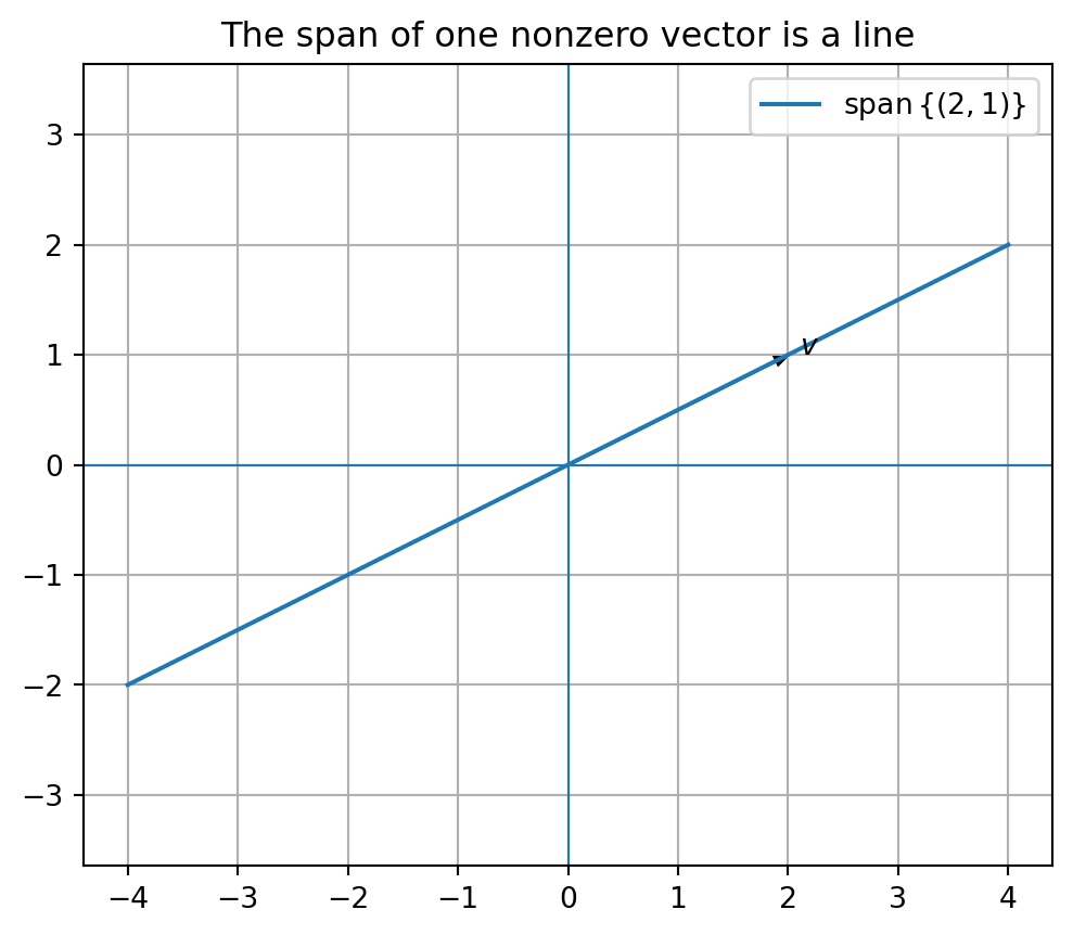
8.7.1 Span of one nonzero vector

Let

\[ v= \begin{bmatrix} 2\\ 1 \end{bmatrix}. \]

Then

\[ \operatorname{span}\{v\} = \left\{ t \begin{bmatrix} 2\\ 1 \end{bmatrix} :t\in\mathbb{R} \right\}. \]

This is a line through the origin.

Every scalar multiple of \(v\) lies on the same line.

import numpy as np
import matplotlib.pyplot as plt

v = np.array([2, 1], dtype=float)
t = np.linspace(-2, 2, 100)
points = np.outer(t, v)

plt.figure(figsize=(6, 5))
plt.plot(points[:, 0], points[:, 1], label=r"$\operatorname{span}\{(2,1)\}$")
plt.arrow(0, 0, v[0], v[1], head_width=0.08, length_includes_head=True)
plt.text(v[0] + 0.1, v[1], "$v$")
plt.axhline(0, linewidth=0.8)
plt.axvline(0, linewidth=0.8)
plt.grid(True)
plt.axis("equal")
plt.legend()
plt.title("The span of one nonzero vector is a line")
plt.show()

8.7.2 Span of two vectors in different directions

Let

\[ v_1= \begin{bmatrix} 1\\ 2 \end{bmatrix}, \qquad v_2= \begin{bmatrix} 1\\ -1 \end{bmatrix}. \]

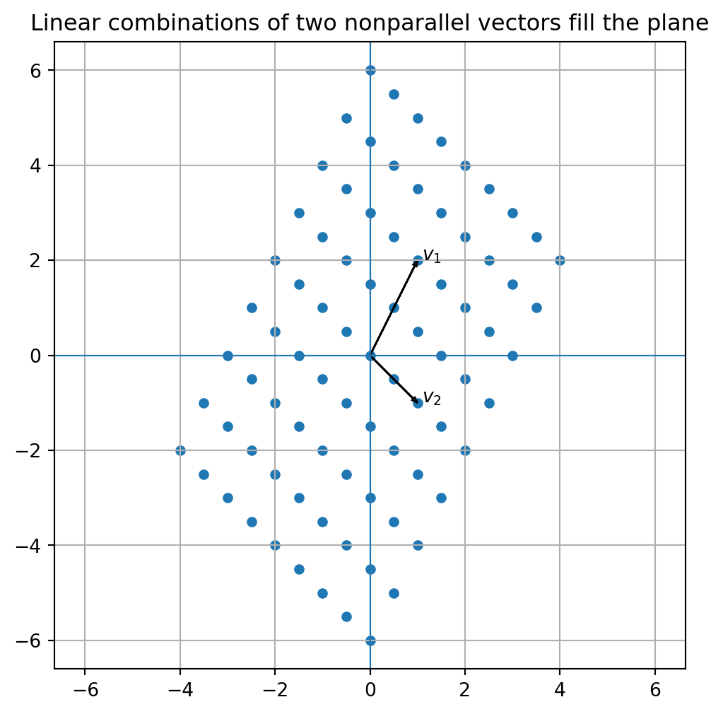
These vectors point in different directions. Their span is all of \(\mathbb{R}^2\).

Why? Because any vector in the plane can be built from them by choosing appropriate coefficients.

v1 = np.array([1, 2], dtype=float)
v2 = np.array([1, -1], dtype=float)

coeffs = np.linspace(-2, 2, 9)
points = []

for c1 in coeffs:
    for c2 in coeffs:
        points.append(c1 * v1 + c2 * v2)

points = np.array(points)

plt.figure(figsize=(6, 6))
plt.scatter(points[:, 0], points[:, 1], s=20)
plt.arrow(0, 0, v1[0], v1[1], head_width=0.08, length_includes_head=True)
plt.arrow(0, 0, v2[0], v2[1], head_width=0.08, length_includes_head=True)
plt.text(v1[0] + 0.1, v1[1], "$v_1$")
plt.text(v2[0] + 0.1, v2[1], "$v_2$")
plt.axhline(0, linewidth=0.8)
plt.axvline(0, linewidth=0.8)
plt.grid(True)
plt.axis("equal")
plt.title("Linear combinations of two nonparallel vectors fill the plane")
plt.show()

8.7.3 Span of two vectors in the same direction

Let

\[ v_1= \begin{bmatrix} 1\\ 2 \end{bmatrix}, \qquad v_2= \begin{bmatrix} 2\\ 4 \end{bmatrix}. \]

Since

\[ v_2=2v_1, \]

the two vectors point in the same direction.

Therefore

\[ \operatorname{span}\{v_1,v_2\} \]

is still only a line through the origin.

Adding a vector that is already a multiple of another vector does not create a new direction.

8.8 6.6 Geometry of span in \(\mathbb{R}^3\)

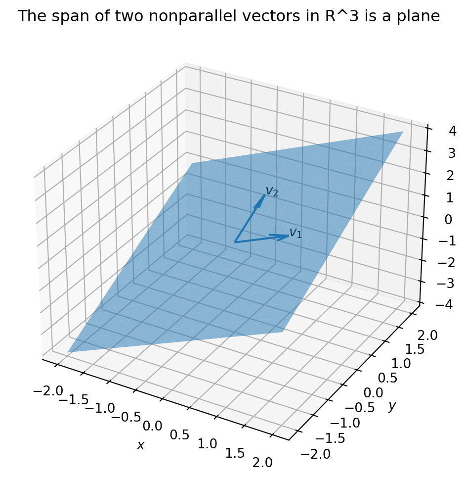
In \(\mathbb{R}^3\), the span of one nonzero vector is a line through the origin.

The span of two nonzero vectors may be:

a line, if the two vectors point in the same or opposite direction,
a plane through the origin, if the two vectors point in different directions.

The span of three vectors may be:

a line,
a plane,
or all of \(\mathbb{R}^3\).

The key question is whether the vectors provide genuinely new directions.

from mpl_toolkits.mplot3d import Axes3D

v1 = np.array([1, 0, 1], dtype=float)
v2 = np.array([0, 1, 1], dtype=float)

s = np.linspace(-2, 2, 15)
t = np.linspace(-2, 2, 15)
S, T = np.meshgrid(s, t)

X = S * v1[0] + T * v2[0]
Y = S * v1[1] + T * v2[1]
Z = S * v1[2] + T * v2[2]

fig = plt.figure(figsize=(7, 6))
ax = fig.add_subplot(111, projection="3d")
ax.plot_surface(X, Y, Z, alpha=0.5)
ax.quiver(0, 0, 0, v1[0], v1[1], v1[2], length=1, normalize=False)
ax.quiver(0, 0, 0, v2[0], v2[1], v2[2], length=1, normalize=False)
ax.text(v1[0], v1[1], v1[2], "$v_1$")
ax.text(v2[0], v2[1], v2[2], "$v_2$")
ax.set_xlabel("$x$")
ax.set_ylabel("$y$")
ax.set_zlabel("$z$")
ax.set_title("The span of two nonparallel vectors in R^3 is a plane")
plt.show()

8.9 6.7 Membership in a span

To determine whether a vector \(b\) lies in the span of \(v_1,\ldots,v_k\), solve the vector equation

\[ c_1v_1+c_2v_2+\cdots+c_kv_k=b. \]

This is a linear system.

If the system is consistent, then \(b\) is in the span.

If the system is inconsistent, then \(b\) is not in the span.

8.9.1 Example

Determine whether

\[ b= \begin{bmatrix} 3\\ 3\\ 4 \end{bmatrix} \]

lies in

\[ \operatorname{span} \left\{ \begin{bmatrix} 1\\ -1\\ 2 \end{bmatrix}, \begin{bmatrix} 2\\ 1\\ 3 \end{bmatrix} \right\}. \]

We need to solve

\[ c_1 \begin{bmatrix} 1\\ -1\\ 2 \end{bmatrix} + c_2 \begin{bmatrix} 2\\ 1\\ 3 \end{bmatrix} = \begin{bmatrix} 3\\ 3\\ 4 \end{bmatrix}. \]

This gives the system

\[ \begin{cases} c_1+2c_2=3,\\ -c_1+c_2=3,\\ 2c_1+3c_2=4. \end{cases} \]

The augmented matrix is

\[ \left[ \begin{array}{cc|c} 1&2&3\\ -1&1&3\\ 2&3&4 \end{array} \right]. \]

Row reduction gives

\[ \left[ \begin{array}{cc|c} 1&0&-1\\ 0&1&2\\ 0&0&0 \end{array} \right]. \]

Therefore

\[ c_1=-1,\qquad c_2=2. \]

\[ b=-1 \begin{bmatrix} 1\\ -1\\ 2 \end{bmatrix} + 2 \begin{bmatrix} 2\\ 1\\ 3 \end{bmatrix}. \]

Thus \(b\) lies in the span.

8.10 6.8 Example: a vector not in the span

Determine whether

\[ b= \begin{bmatrix} 0\\ 1\\ 2 \end{bmatrix} \]

lies in

\[ \operatorname{span} \left\{ \begin{bmatrix} 1\\ -1\\ 2 \end{bmatrix}, \begin{bmatrix} 2\\ 1\\ 3 \end{bmatrix} \right\}. \]

Solve

\[ c_1 \begin{bmatrix} 1\\ -1\\ 2 \end{bmatrix} + c_2 \begin{bmatrix} 2\\ 1\\ 3 \end{bmatrix} = \begin{bmatrix} 0\\ 1\\ 2 \end{bmatrix}. \]

This gives

\[ \left[ \begin{array}{cc|c} 1&2&0\\ -1&1&1\\ 2&3&2 \end{array} \right]. \]

Row reduction produces a contradiction:

\[ \left[ \begin{array}{cc|c} 1&0&3\\ 0&1&-2\\ 0&0&5 \end{array} \right]. \]

The last row means

\[ 0=5. \]

Therefore the system is inconsistent, and \(b\) does not lie in the span.

8.11 6.9 Span and the equation \(Ax=b\)

Let

\[ A= \begin{bmatrix} |&|&&|\\ a_1&a_2&\cdots&a_n\\ |&|&&| \end{bmatrix}. \]

Then

\[ Ax=b \]

means

\[ x_1a_1+x_2a_2+\cdots+x_na_n=b. \]

Therefore:

Span interpretation of \(Ax=b\)

The system \(Ax=b\) is consistent if and only if \(b\) is in the span of the columns of \(A\).

That is,

\[ Ax=b \text{ has a solution} \]

if and only if

\[ b\in \operatorname{span}\{a_1,a_2,\ldots,a_n\}. \]

This is one of the most important translations in linear algebra.

8.12 6.10 Row picture versus column picture

Consider

\[ A= \begin{bmatrix} 1&1\\ 2&-1 \end{bmatrix}, \qquad b= \begin{bmatrix} 5\\ 1 \end{bmatrix}. \]

The system

\[ Ax=b \]

\[ \begin{cases} x_1+x_2=5,\\ 2x_1-x_2=1. \end{cases} \]

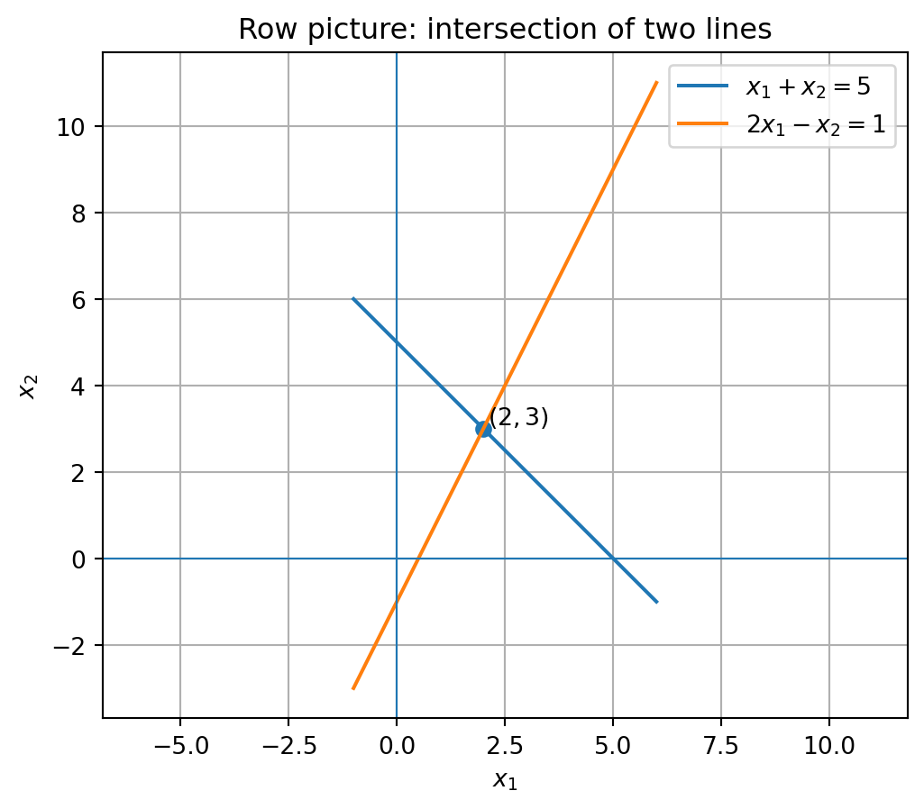
8.12.1 Row picture

Each row gives a line:

\[ x_1+x_2=5, \]

\[ 2x_1-x_2=1. \]

The solution is the intersection point:

\[ (x_1,x_2)=(2,3). \]

8.12.2 Column picture

The columns are

\[ a_1= \begin{bmatrix} 1\\ 2 \end{bmatrix}, \qquad a_2= \begin{bmatrix} 1\\ -1 \end{bmatrix}. \]

The equation becomes

\[ x_1a_1+x_2a_2=b. \]

With \(x_1=2\) and \(x_2=3\),

\[ 2 \begin{bmatrix} 1\\ 2 \end{bmatrix} + 3 \begin{bmatrix} 1\\ -1 \end{bmatrix} = \begin{bmatrix} 5\\ 1 \end{bmatrix}. \]

The row picture asks:

Where do the equations intersect?

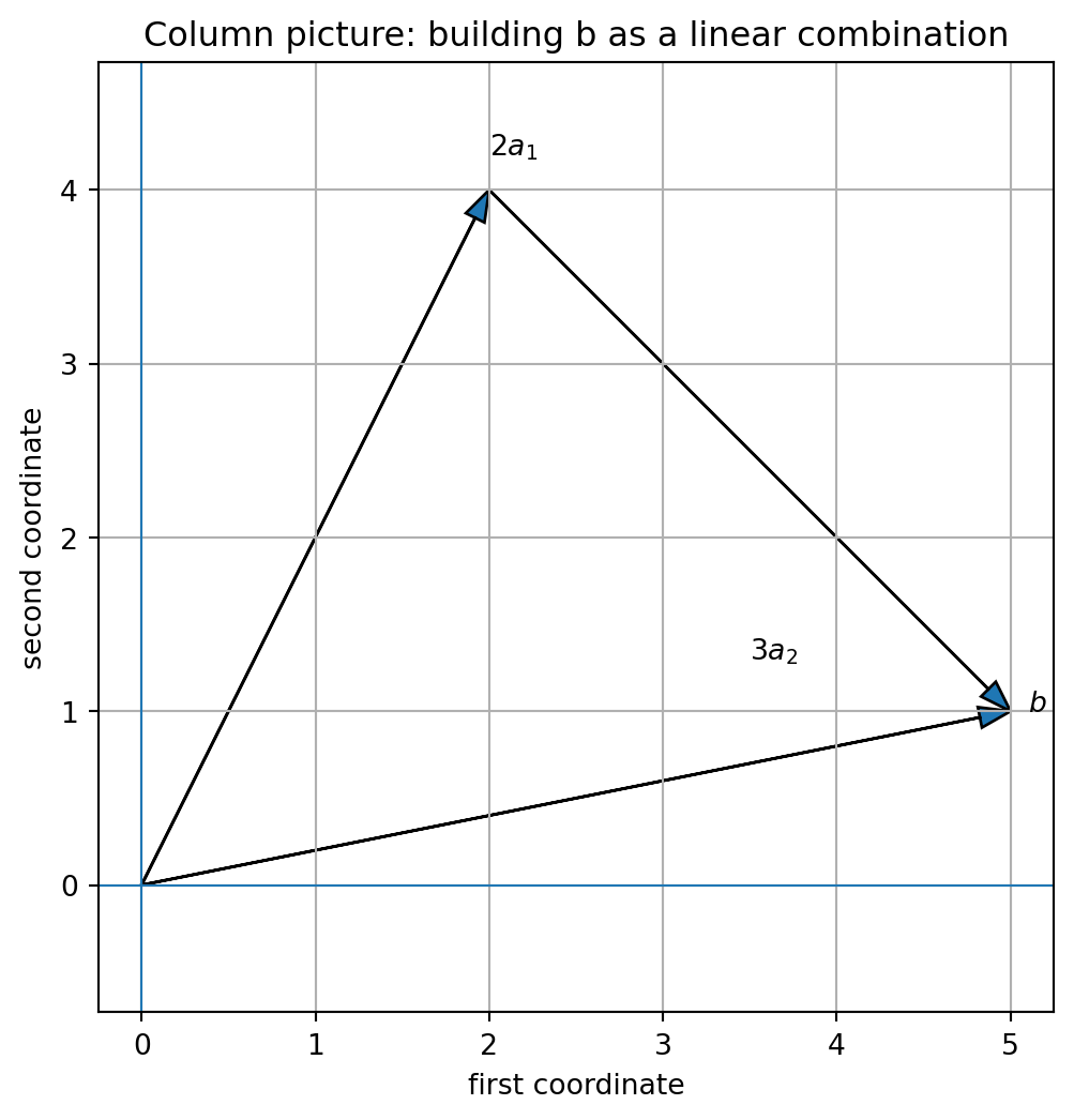
The column picture asks:

How do we build \(b\) from the columns of \(A\)?

Both pictures are correct. They emphasize different aspects of the same problem.

# Row picture for the system x1 + x2 = 5, 2x1 - x2 = 1
x = np.linspace(-1, 6, 300)
y1 = 5 - x
y2 = 2*x - 1

plt.figure(figsize=(6, 5))
plt.plot(x, y1, label="$x_1+x_2=5$")
plt.plot(x, y2, label="$2x_1-x_2=1$")
plt.scatter([2], [3])
plt.text(2.1, 3.1, "$(2,3)$")
plt.axhline(0, linewidth=0.8)
plt.axvline(0, linewidth=0.8)
plt.grid(True)
plt.axis("equal")
plt.legend()
plt.title("Row picture: intersection of two lines")
plt.xlabel("$x_1$")
plt.ylabel("$x_2$")
plt.show()

# Column picture for b = 2 a1 + 3 a2
a1 = np.array([1, 2], dtype=float)
a2 = np.array([1, -1], dtype=float)
b = 2*a1 + 3*a2

plt.figure(figsize=(6, 6))
plt.arrow(0, 0, 2*a1[0], 2*a1[1], head_width=0.12, length_includes_head=True)
plt.arrow(2*a1[0], 2*a1[1], 3*a2[0], 3*a2[1], head_width=0.12, length_includes_head=True)
plt.arrow(0, 0, b[0], b[1], head_width=0.12, length_includes_head=True)
plt.text(2*a1[0], 2*a1[1] + 0.2, "$2a_1$")
plt.text(b[0] - 1.5, b[1] + 0.3, "$3a_2$")
plt.text(b[0] + 0.1, b[1], "$b$")
plt.axhline(0, linewidth=0.8)
plt.axvline(0, linewidth=0.8)
plt.grid(True)
plt.axis("equal")
plt.title("Column picture: building b as a linear combination")
plt.xlabel("first coordinate")
plt.ylabel("second coordinate")
plt.show()

8.13 6.11 Spanning \(\mathbb{R}^n\)

A set of vectors spans \(\mathbb{R}^n\) if every vector in \(\mathbb{R}^n\) can be written as a linear combination of them.

For example, the standard basis vectors

\[ e_1= \begin{bmatrix} 1\\ 0\\ 0 \end{bmatrix}, \qquad e_2= \begin{bmatrix} 0\\ 1\\ 0 \end{bmatrix}, \qquad e_3= \begin{bmatrix} 0\\ 0\\ 1 \end{bmatrix} \]

span \(\mathbb{R}^3\), because every vector

\[ \begin{bmatrix} x\\ y\\ z \end{bmatrix} \]

can be written as

\[ x e_1+y e_2+z e_3. \]

That is,

\[ \begin{bmatrix} x\\ y\\ z \end{bmatrix} = x \begin{bmatrix} 1\\ 0\\ 0 \end{bmatrix} + y \begin{bmatrix} 0\\ 1\\ 0 \end{bmatrix} + z \begin{bmatrix} 0\\ 0\\ 1 \end{bmatrix}. \]

8.14 6.12 When do vectors span \(\mathbb{R}^2\)?

Two vectors in \(\mathbb{R}^2\) span \(\mathbb{R}^2\) if they are not multiples of each other.

Example:

\[ \begin{bmatrix} 1\\ 2 \end{bmatrix}, \qquad \begin{bmatrix} 1\\ -1 \end{bmatrix} \]

span \(\mathbb{R}^2\).

But

\[ \begin{bmatrix} 1\\ 2 \end{bmatrix}, \qquad \begin{bmatrix} 2\\ 4 \end{bmatrix} \]

do not span \(\mathbb{R}^2\), because the second vector is a multiple of the first.

Their span is only a line.

8.15 6.13 When do vectors span \(\mathbb{R}^3\)?

Three vectors in \(\mathbb{R}^3\) span \(\mathbb{R}^3\) if they provide three independent directions.

If all three vectors lie in the same plane through the origin, then they do not span \(\mathbb{R}^3\).

If they do not all lie in one plane through the origin, then they span \(\mathbb{R}^3\).

Computationally, put the vectors as columns of a matrix and row reduce.

If there is a pivot in every row, the columns span \(\mathbb{R}^3\).

This row-reduction criterion will be developed more fully in the next chapters.

8.16 6.14 Span of the columns and column space preview

The span of the columns of a matrix is so important that it has a name.

Definition: column space

The column space of a matrix \(A\) is the span of the columns of \(A\).

It is written as

\[ \operatorname{Col}(A). \]

\[ A= \begin{bmatrix} |&|&&|\\ a_1&a_2&\cdots&a_n\\ |&|&&| \end{bmatrix}, \]

then

\[ \operatorname{Col}(A)=\operatorname{span}\{a_1,a_2,\ldots,a_n\}. \]

The equation

\[ Ax=b \]

is consistent if and only if

\[ b\in \operatorname{Col}(A). \]

We will study column spaces in detail later.

8.17 6.15 Linear combinations as data models

A linear combination is also a simple model-building idea.

Suppose a signal \(b\) is built from basic patterns \(v_1,v_2,v_3\):

\[ b=c_1v_1+c_2v_2+c_3v_3. \]

Then the coefficients \(c_1,c_2,c_3\) tell us how much of each pattern is used.

This idea appears in:

image reconstruction,
audio processing,
regression,
feature engineering,
recommendation systems,
principal component analysis,
neural network layers.

In each case, we ask:

Can a complicated object be built from simpler building blocks?

Linear combinations provide the first mathematical language for that question.

8.18 6.16 Python: testing span membership with SymPy

Let

\[ v_1= \begin{bmatrix} 1\\ -1\\ 2 \end{bmatrix}, \qquad v_2= \begin{bmatrix} 2\\ 1\\ 3 \end{bmatrix}, \qquad b= \begin{bmatrix} 3\\ 3\\ 4 \end{bmatrix}. \]

We test whether \(b\) lies in the span of \(v_1\) and \(v_2\) by solving

\[ c_1v_1+c_2v_2=b. \]

import sympy as sp

A = sp.Matrix([
    [1, 2],
    [-1, 1],
    [2, 3]
])

b = sp.Matrix([3, 3, 4])

aug = A.row_join(b)
aug.rref()

(Matrix([
 [1, 0, -1],
 [0, 1,  2],
 [0, 0,  0]]),
 (0, 1))

The last row is not contradictory, so \(b\) is in the span.

The solution is

\[ c_1=-1,\qquad c_2=2. \]

8.19 6.17 Python: inconsistent span membership

Now test

\[ b= \begin{bmatrix} 0\\ 1\\ 2 \end{bmatrix}. \]

b2 = sp.Matrix([0, 1, 2])
aug2 = A.row_join(b2)
aug2.rref()

(Matrix([
 [1, 0, 0],
 [0, 1, 0],
 [0, 0, 1]]),
 (0, 1, 2))

The rref contains a contradiction, so \(b\) is not in the span.

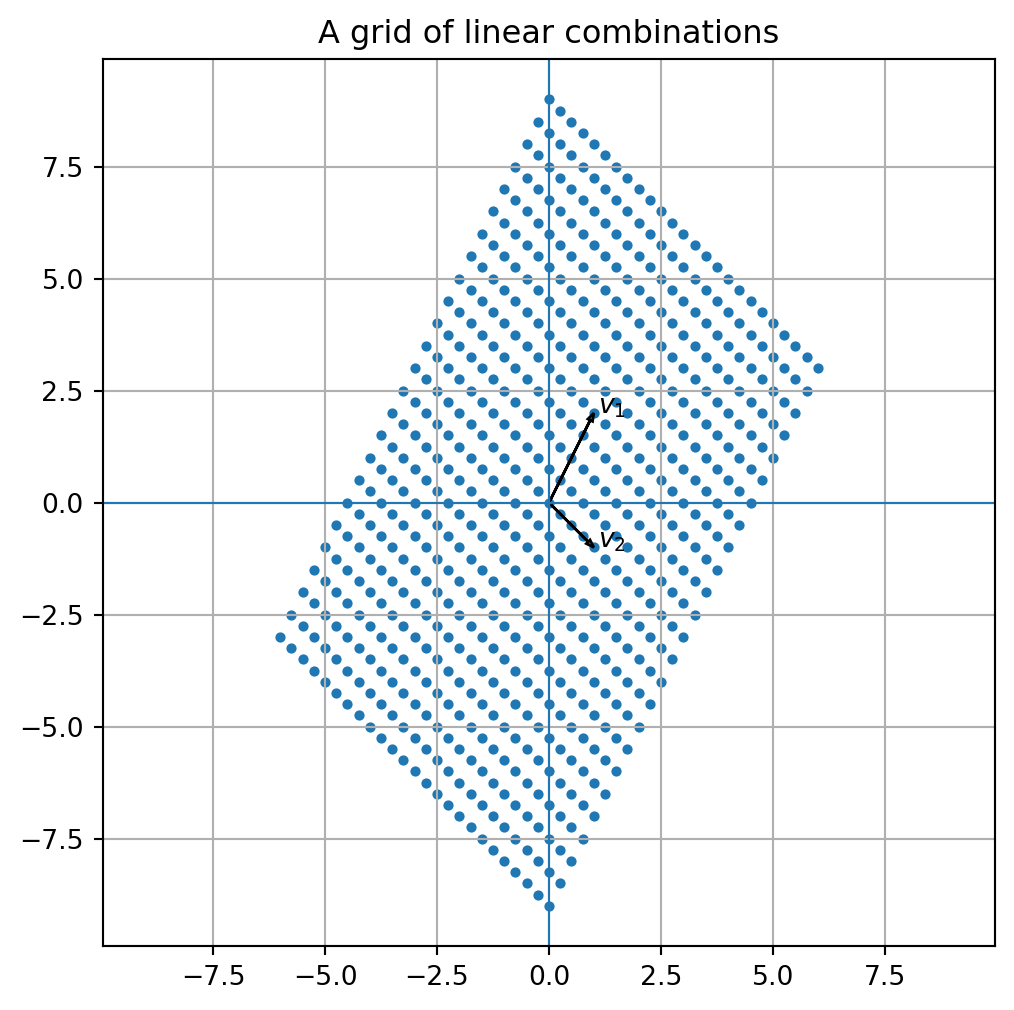
8.20 6.18 Python: many linear combinations

We can generate many linear combinations of two vectors.

v1 = np.array([1, 2], dtype=float)
v2 = np.array([1, -1], dtype=float)

coeffs = np.linspace(-3, 3, 25)
points = []

for c1 in coeffs:
    for c2 in coeffs:
        points.append(c1*v1 + c2*v2)

points = np.array(points)

plt.figure(figsize=(6, 6))
plt.scatter(points[:, 0], points[:, 1], s=8)
plt.arrow(0, 0, v1[0], v1[1], head_width=0.12, length_includes_head=True)
plt.arrow(0, 0, v2[0], v2[1], head_width=0.12, length_includes_head=True)
plt.text(v1[0] + 0.1, v1[1], "$v_1$")
plt.text(v2[0] + 0.1, v2[1], "$v_2$")
plt.axhline(0, linewidth=0.8)
plt.axvline(0, linewidth=0.8)
plt.grid(True)
plt.axis("equal")
plt.title("A grid of linear combinations")
plt.show()

The plotted points form a transformed grid. This is an early picture of how matrices transform space.

8.21 6.19 Algorithm: testing whether \(b\) is in a span

Algorithm: membership in a span

To determine whether

\[ b\in \operatorname{span}\{v_1,\ldots,v_k\}, \]

do the following:

Form the matrix

\[ A=\begin{bmatrix}v_1&v_2&\cdots&v_k\end{bmatrix}. \]

Solve

\[ Ax=b. \]

Equivalently, row reduce the augmented matrix

\[ [A\mid b]. \]

If the system is consistent, then \(b\) is in the span.
If the system is inconsistent, then \(b\) is not in the span.

8.22 6.20 Common mistakes

8.22.1 Mistake 1: confusing a set of vectors with its span

The set

\[ \{v_1,v_2\} \]

contains only two vectors.

The span

\[ \operatorname{span}\{v_1,v_2\} \]

contains all linear combinations of those vectors, usually infinitely many vectors.

8.22.2 Mistake 2: forgetting scalar multiples

If \(v\) is in a span, then every scalar multiple of \(v\) is also in the span.

8.22.3 Mistake 3: thinking two vectors in \(\mathbb{R}^3\) can span all of \(\mathbb{R}^3\)

Two vectors in \(\mathbb{R}^3\) can span at most a plane. They cannot span all of \(\mathbb{R}^3\).

8.22.4 Mistake 4: only checking visually

Graphs help build intuition, but row reduction gives the exact answer.

8.22.5 Mistake 5: mixing row and column pictures

The row picture describes equations as intersections.

The column picture describes the right-hand side as a linear combination of columns.

Both are useful, but they answer different visual questions.

8.23 6.21 Chapter summary

A linear combination of vectors \(v_1,\ldots,v_k\) is

\[ c_1v_1+\cdots+c_kv_k. \]

The span of vectors is the set of all their linear combinations:

\[ \operatorname{span}\{v_1,\ldots,v_k\} = \{c_1v_1+\cdots+c_kv_k:c_i\in\mathbb{R}\}. \]

Matrix-vector multiplication is a linear combination of columns:

\[ Ax=x_1a_1+\cdots+x_na_n. \]

The system \(Ax=b\) is consistent if and only if \(b\) lies in the span of the columns of \(A\).

The row picture views a system as intersections of equations.

The column picture views a system as building \(b\) from columns.

The column space of \(A\) is

\[ \operatorname{Col}(A)=\operatorname{span}\{\text{columns of }A\}. \]

Span is the first major step toward subspaces, bases, dimension, rank, and data representation.

8.24 Exercises

8.24.1 A. Linear combinations

Compute each linear combination.

\[ 2 \begin{bmatrix} 1\\ 2 \end{bmatrix} + 3 \begin{bmatrix} 1\\ -1 \end{bmatrix} \]

\[ -1 \begin{bmatrix} 1\\ -1\\ 2 \end{bmatrix} + 2 \begin{bmatrix} 2\\ 1\\ 3 \end{bmatrix} \]

\[ 4 \begin{bmatrix} 1\\ 0\\ 0 \end{bmatrix} - 2 \begin{bmatrix} 0\\ 1\\ 0 \end{bmatrix} + 5 \begin{bmatrix} 0\\ 0\\ 1 \end{bmatrix} \]

\[ s \begin{bmatrix} 2\\ 1 \end{bmatrix} + t \begin{bmatrix} -1\\ 3 \end{bmatrix} \]

where \(s=2\) and \(t=-1\).

8.24.2 B. Describe the span geometrically

Describe each span geometrically.

\[ \operatorname{span} \left\{ \begin{bmatrix} 2\\ 1 \end{bmatrix} \right\} \]

\[ \operatorname{span} \left\{ \begin{bmatrix} 1\\ 2 \end{bmatrix}, \begin{bmatrix} 2\\ 4 \end{bmatrix} \right\} \]

\[ \operatorname{span} \left\{ \begin{bmatrix} 1\\ 2 \end{bmatrix}, \begin{bmatrix} 1\\ -1 \end{bmatrix} \right\} \]

\[ \operatorname{span} \left\{ \begin{bmatrix} 1\\ 0\\ 1 \end{bmatrix}, \begin{bmatrix} 0\\ 1\\ 1 \end{bmatrix} \right\} \]

8.24.3 C. Membership in a span

Determine whether \(b\) lies in the span of the given vectors. If it does, write \(b\) as a linear combination.

\[ b= \begin{bmatrix} 5\\ 1 \end{bmatrix}, \qquad v_1= \begin{bmatrix} 1\\ 2 \end{bmatrix}, \qquad v_2= \begin{bmatrix} 1\\ -1 \end{bmatrix}. \]

\[ b= \begin{bmatrix} 3\\ 3\\ 4 \end{bmatrix}, \qquad v_1= \begin{bmatrix} 1\\ -1\\ 2 \end{bmatrix}, \qquad v_2= \begin{bmatrix} 2\\ 1\\ 3 \end{bmatrix}. \]

\[ b= \begin{bmatrix} 0\\ 1\\ 2 \end{bmatrix}, \qquad v_1= \begin{bmatrix} 1\\ -1\\ 2 \end{bmatrix}, \qquad v_2= \begin{bmatrix} 2\\ 1\\ 3 \end{bmatrix}. \]

\[ b= \begin{bmatrix} 1\\ 2\\ 3 \end{bmatrix}, \qquad v_1= \begin{bmatrix} 1\\ 0\\ 1 \end{bmatrix}, \qquad v_2= \begin{bmatrix} 0\\ 1\\ 1 \end{bmatrix}, \qquad v_3= \begin{bmatrix} 1\\ 1\\ 0 \end{bmatrix}. \]

8.24.4 D. Column picture

For each system, write the column-picture equation.

\[ \begin{bmatrix} 1&1\\ 2&-1 \end{bmatrix} \begin{bmatrix} x_1\\ x_2 \end{bmatrix} = \begin{bmatrix} 5\\ 1 \end{bmatrix} \]

\[ \begin{bmatrix} 1&0&1\\ 0&1&1 \end{bmatrix} \begin{bmatrix} x_1\\ x_2\\ x_3 \end{bmatrix} = \begin{bmatrix} 3\\ 4 \end{bmatrix} \]

\[ \begin{bmatrix} 1&2\\ -1&1\\ 2&3 \end{bmatrix} \begin{bmatrix} c_1\\ c_2 \end{bmatrix} = \begin{bmatrix} 3\\ 3\\ 4 \end{bmatrix} \]

8.24.5 E. Spanning \(\mathbb{R}^n\)

Determine whether the given vectors span the indicated space.

\[ \left\{ \begin{bmatrix} 1\\ 0 \end{bmatrix}, \begin{bmatrix} 0\\ 1 \end{bmatrix} \right\} \]

in \(\mathbb{R}^2\).

\[ \left\{ \begin{bmatrix} 1\\ 2 \end{bmatrix}, \begin{bmatrix} 2\\ 4 \end{bmatrix} \right\} \]

in \(\mathbb{R}^2\).

\[ \left\{ \begin{bmatrix} 1\\ 0\\ 0 \end{bmatrix}, \begin{bmatrix} 0\\ 1\\ 0 \end{bmatrix} \right\} \]

in \(\mathbb{R}^3\).

\[ \left\{ \begin{bmatrix} 1\\ 0\\ 0 \end{bmatrix}, \begin{bmatrix} 0\\ 1\\ 0 \end{bmatrix}, \begin{bmatrix} 0\\ 0\\ 1 \end{bmatrix} \right\} \]

in \(\mathbb{R}^3\).

8.24.6 F. Python exercises

Use NumPy to generate and plot scalar multiples of

\[ v= \begin{bmatrix} 2\\ 1 \end{bmatrix}. \]

Use NumPy to generate many linear combinations of

\[ v_1= \begin{bmatrix} 1\\ 2 \end{bmatrix}, \qquad v_2= \begin{bmatrix} 1\\ -1 \end{bmatrix}. \]

Use SymPy to determine whether

\[ b= \begin{bmatrix} 3\\ 3\\ 4 \end{bmatrix} \]

lies in the span of

\[ v_1= \begin{bmatrix} 1\\ -1\\ 2 \end{bmatrix}, \qquad v_2= \begin{bmatrix} 2\\ 1\\ 3 \end{bmatrix}. \]

Use SymPy to determine whether

\[ b= \begin{bmatrix} 0\\ 1\\ 2 \end{bmatrix} \]

lies in the same span.

Create a \(3\)D plot of the span of

\[ v_1= \begin{bmatrix} 1\\ 0\\ 1 \end{bmatrix}, \qquad v_2= \begin{bmatrix} 0\\ 1\\ 1 \end{bmatrix}. \]

8.24.7 G. Reflection

Write a short paragraph answering each question.

What is the difference between a set of vectors and its span?
Why is \(Ax=b\) really a question about the span of the columns of \(A\)?
How does the row picture differ from the column picture?
Why is span important for data representation?

8.25 AI-age connection

Linear combinations are everywhere in modern computation. A machine learning model often builds predictions from weighted combinations of features. A neural network layer computes matrix-vector products, which are linear combinations of columns or rows. A signal can be approximated by combining basis patterns. A recommendation system may represent a user as a combination of preference vectors. Span is the mathematical language of what can be built from available building blocks.