Opening question
A vector is an object, but its coordinates depend on the basis we use to describe it.
For example, in the standard basis of \(\mathbb{R}^2\) ,
\[
b=
\begin{bmatrix}
3\\
1
\end{bmatrix}
\]
means
\[
b=3e_1+1e_2.
\]
But if we use the basis
\[
\mathcal{B}=
\left\{
\begin{bmatrix}
1\\
1
\end{bmatrix},
\begin{bmatrix}
1\\
-1
\end{bmatrix}
\right\},
\]
then the same vector has coordinates
\[
[b]_{\mathcal{B}}
=
\begin{bmatrix}
2\\
1
\end{bmatrix},
\]
because
\[
b=
2
\begin{bmatrix}
1\\
1
\end{bmatrix}
+
1
\begin{bmatrix}
1\\
-1
\end{bmatrix}.
\]
The vector did not change. Only the coordinate system changed.
The central question of this chapter is:
How do we translate vectors and matrices from one basis to another?
Learning goals
After studying this chapter, you should be able to:
Explain the difference between a vector and its coordinates.
Compute coordinates relative to a nonstandard basis.
Build the basis matrix associated with a basis.
Convert from basis coordinates to standard coordinates.
Convert from standard coordinates to basis coordinates.
Define and compute change-of-basis matrices.
Change coordinates between two nonstandard bases.
Understand how matrix representations depend on basis.
Recognize similarity as change of coordinates for square matrices.
Use Python to visualize and compute coordinate changes.
9.1 Vectors versus coordinates
A vector is a geometric or data object.
Coordinates are a description of that object relative to a chosen basis.
In the standard basis of \(\mathbb{R}^2\) ,
\[
e_1=
\begin{bmatrix}
1\\
0
\end{bmatrix},
\qquad
e_2=
\begin{bmatrix}
0\\
1
\end{bmatrix},
\]
the vector
\[
b=
\begin{bmatrix}
3\\
1
\end{bmatrix}
\]
means
\[
b=3e_1+1e_2.
\]
But relative to another basis, the same vector may have different coordinates.
This distinction is fundamental:
A vector is the object. Coordinates are its address in a basis.
9.2 Coordinates relative to a basis
Let
\[
\mathcal{B}=\{v_1,v_2,\ldots,v_n\}
\]
be a basis for \(\mathbb{R}^n\) .
For every vector \(x\in\mathbb{R}^n\) , there is a unique choice of scalars
\[
c_1,c_2,\ldots,c_n
\]
such that
\[
x=c_1v_1+c_2v_2+\cdots+c_nv_n.
\]
The coordinate vector of \(x\) relative to the basis \(\mathcal{B}\) is
\[
[x]_{\mathcal{B}}
=
\begin{bmatrix}
c_1\\
c_2\\
\vdots\\
c_n
\end{bmatrix}.
\]
The vector \([x]_{\mathcal{B}}\) does not list the standard coordinates of \(x\) . It lists the weights needed to build \(x\) from the basis vectors in \(\mathcal{B}\) .
9.3 First example
Let
\[
\mathcal{B}=
\left\{
v_1=
\begin{bmatrix}
1\\
1
\end{bmatrix},
\quad
v_2=
\begin{bmatrix}
1\\
-1
\end{bmatrix}
\right\}.
\]
Find the coordinates of
\[
b=
\begin{bmatrix}
3\\
1
\end{bmatrix}
\]
relative to \(\mathcal{B}\) .
We solve
\[
c_1
\begin{bmatrix}
1\\
1
\end{bmatrix}
+
c_2
\begin{bmatrix}
1\\
-1
\end{bmatrix}
=
\begin{bmatrix}
3\\
1
\end{bmatrix}.
\]
This gives the system
\[
c_1+c_2=3,
\]
\[
c_1-c_2=1.
\]
Adding the equations gives
\[
2c_1=4,
\]
so
\[
c_1=2.
\]
Then
\[
c_2=1.
\]
Therefore
\[
[b]_{\mathcal{B}}
=
\begin{bmatrix}
2\\
1
\end{bmatrix}.
\]
This means
\[
b=2v_1+1v_2.
\]
9.4 The basis matrix
Let
\[
\mathcal{B}=\{v_1,v_2,\ldots,v_n\}
\]
be a basis for \(\mathbb{R}^n\) .
The basis matrix associated with \(\mathcal{B}\) is
\[
P_{\mathcal{B}}
=
\begin{bmatrix}
|&|&&|\\
v_1&v_2&\cdots&v_n\\
|&|&&|
\end{bmatrix}.
\]
That is, the basis vectors are placed as columns.
If
\[
[x]_{\mathcal{B}}
=
\begin{bmatrix}
c_1\\
c_2\\
\vdots\\
c_n
\end{bmatrix},
\]
then
\[
x=P_{\mathcal{B}}[x]_{\mathcal{B}}.
\]
This equation converts basis coordinates into standard coordinates.
\[
x=P_{\mathcal{B}}[x]_{\mathcal{B}}.
\]
9.5 Standard coordinates to basis coordinates
If
\[
x=P_{\mathcal{B}}[x]_{\mathcal{B}},
\]
then to find \([x]_{\mathcal{B}}\) , solve the system
\[
P_{\mathcal{B}}c=x.
\]
Since \(\mathcal{B}\) is a basis, \(P_{\mathcal{B}}\) is invertible.
Thus
\[
[x]_{\mathcal{B}}=P_{\mathcal{B}}^{-1}x.
\]
\[
[x]_{\mathcal{B}}=P_{\mathcal{B}}^{-1}x.
\]
This formula is simple but important. It says that coordinate conversion is a linear transformation.
9.6 Example using the basis matrix
For
\[
\mathcal{B}=
\left\{
\begin{bmatrix}
1\\
1
\end{bmatrix},
\begin{bmatrix}
1\\
-1
\end{bmatrix}
\right\},
\]
the basis matrix is
\[
P_{\mathcal{B}}
=
\begin{bmatrix}
1&1\\
1&-1
\end{bmatrix}.
\]
If
\[
[b]_{\mathcal{B}}=
\begin{bmatrix}
2\\
1
\end{bmatrix},
\]
then
\[
b=P_{\mathcal{B}}[b]_{\mathcal{B}}
=
\begin{bmatrix}
1&1\\
1&-1
\end{bmatrix}
\begin{bmatrix}
2\\
1
\end{bmatrix}
=
\begin{bmatrix}
3\\
1
\end{bmatrix}.
\]
Conversely,
\[
[b]_{\mathcal{B}}
=
P_{\mathcal{B}}^{-1}b.
\]
Since
\[
P_{\mathcal{B}}^{-1}
=
\frac12
\begin{bmatrix}
1&1\\
1&-1
\end{bmatrix},
\]
we get
\[
[b]_{\mathcal{B}}
=
\frac12
\begin{bmatrix}
1&1\\
1&-1
\end{bmatrix}
\begin{bmatrix}
3\\
1
\end{bmatrix}
=
\begin{bmatrix}
2\\
1
\end{bmatrix}.
\]
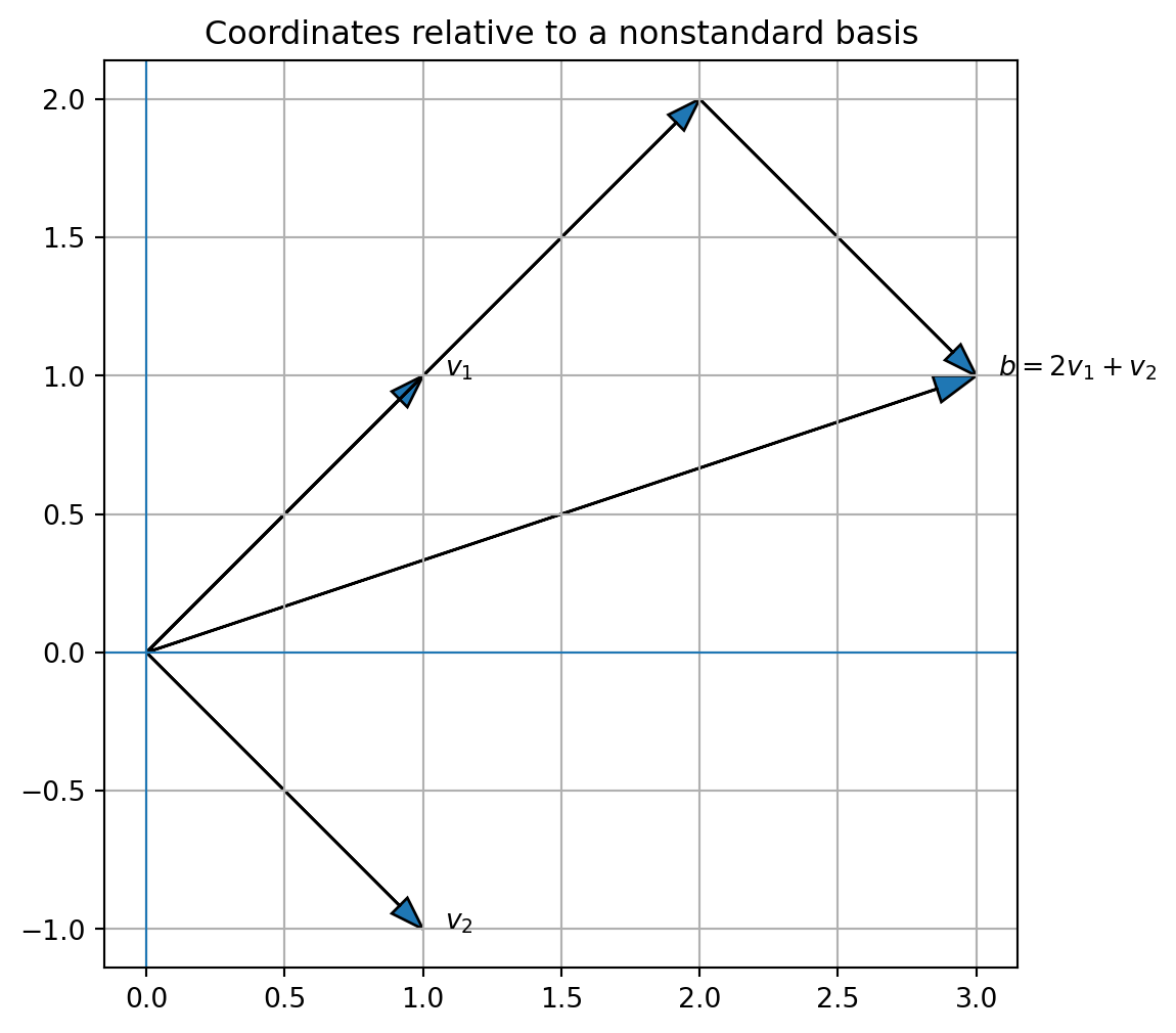
9.7 Geometric interpretation in \(\mathbb{R}^2\)
The standard basis uses horizontal and vertical axes.
A nonstandard basis uses new coordinate axes determined by its basis vectors.
For example,
\[
v_1=
\begin{bmatrix}
1\\
1
\end{bmatrix},
\qquad
v_2=
\begin{bmatrix}
1\\
-1
\end{bmatrix}
\]
form diagonal axes.
The coordinate vector
\[
[b]_{\mathcal{B}}
=
\begin{bmatrix}
2\\
1
\end{bmatrix}
\]
means:
move \(2\) units in the \(v_1\) direction,
move \(1\) unit in the \(v_2\) direction.
The resulting vector is
\[
b=
\begin{bmatrix}
3\\
1
\end{bmatrix}.
\]
import numpy as npimport matplotlib.pyplot as plt= np.array([1 , 1 ], dtype= float )= np.array([1 , - 1 ], dtype= float )= 2 * v1 + 1 * v2= (6 , 6 ))0 , 0 , v1[0 ], v1[1 ], head_width= 0.08 , length_includes_head= True )0 , 0 , v2[0 ], v2[1 ], head_width= 0.08 , length_includes_head= True )0 , 0 , b[0 ], b[1 ], head_width= 0.1 , length_includes_head= True )0 , 0 , 2 * v1[0 ], 2 * v1[1 ], head_width= 0.08 , length_includes_head= True )2 * v1[0 ], 2 * v1[1 ], v2[0 ], v2[1 ], head_width= 0.08 , length_includes_head= True )0 ]+ 0.08 , v1[1 ], "$v_1$" )0 ]+ 0.08 , v2[1 ], "$v_2$" )0 ]+ 0.08 , b[1 ], "$b=2v_1+v_2$" )0 , linewidth= 0.8 )0 , linewidth= 0.8 )True )"equal" )"Coordinates relative to a nonstandard basis" )
9.8 Change of basis from one basis to another
Now suppose we have two bases of \(\mathbb{R}^n\) :
\[
\mathcal{B}=\{b_1,\ldots,b_n\},
\qquad
\mathcal{C}=\{c_1,\ldots,c_n\}.
\]
A vector \(x\) has coordinates \([x]_{\mathcal{B}}\) in the \(\mathcal{B}\) basis and coordinates \([x]_{\mathcal{C}}\) in the \(\mathcal{C}\) basis.
We want to convert between them.
Using standard coordinates,
\[
x=P_{\mathcal{B}}[x]_{\mathcal{B}}
\]
and
\[
x=P_{\mathcal{C}}[x]_{\mathcal{C}}.
\]
Therefore
\[
P_{\mathcal{C}}[x]_{\mathcal{C}}
=
P_{\mathcal{B}}[x]_{\mathcal{B}}.
\]
Multiply by \(P_{\mathcal{C}}^{-1}\) :
\[
[x]_{\mathcal{C}}
=
P_{\mathcal{C}}^{-1}P_{\mathcal{B}}[x]_{\mathcal{B}}.
\]
The matrix that converts \(\mathcal{B}\) -coordinates to \(\mathcal{C}\) -coordinates is
\[
P_{\mathcal{C}\leftarrow\mathcal{B}}
=
P_{\mathcal{C}}^{-1}P_{\mathcal{B}}.
\]
Thus
\[
[x]_{\mathcal{C}}
=
P_{\mathcal{C}\leftarrow\mathcal{B}}[x]_{\mathcal{B}}.
\]
The notation \(P_{\mathcal{C}\leftarrow\mathcal{B}}\) means:
input coordinates are in basis \(\mathcal{B}\) , output coordinates are in basis \(\mathcal{C}\) .
9.9 Example: changing between two bases
Let
\[
\mathcal{B}=
\left\{
\begin{bmatrix}1\\1\end{bmatrix},
\begin{bmatrix}1\\-1\end{bmatrix}
\right\}
\]
and
\[
\mathcal{C}=
\left\{
\begin{bmatrix}2\\1\end{bmatrix},
\begin{bmatrix}1\\1\end{bmatrix}
\right\}.
\]
Suppose
\[
[x]_{\mathcal{B}}
=
\begin{bmatrix}
2\\
1
\end{bmatrix}.
\]
First find the standard vector:
\[
x=P_{\mathcal{B}}[x]_{\mathcal{B}}
=
\begin{bmatrix}
1&1\\
1&-1
\end{bmatrix}
\begin{bmatrix}
2\\
1
\end{bmatrix}
=
\begin{bmatrix}
3\\
1
\end{bmatrix}.
\]
Now find \(\mathcal{C}\) -coordinates. We solve
\[
P_{\mathcal{C}}[x]_{\mathcal{C}}=x,
\]
where
\[
P_{\mathcal{C}}=
\begin{bmatrix}
2&1\\
1&1
\end{bmatrix}.
\]
Let
\[
[x]_{\mathcal{C}}
=
\begin{bmatrix}
u\\
v
\end{bmatrix}.
\]
Then
\[
2u+v=3,
\]
\[
u+v=1.
\]
Subtracting gives
\[
u=2,
\]
and then
\[
v=-1.
\]
Therefore
\[
[x]_{\mathcal{C}}
=
\begin{bmatrix}
2\\
-1
\end{bmatrix}.
\]
So the same vector can be described as
\[
[x]_{\mathcal{B}}=
\begin{bmatrix}
2\\
1
\end{bmatrix}
\]
or as
\[
[x]_{\mathcal{C}}=
\begin{bmatrix}
2\\
-1
\end{bmatrix}.
\]
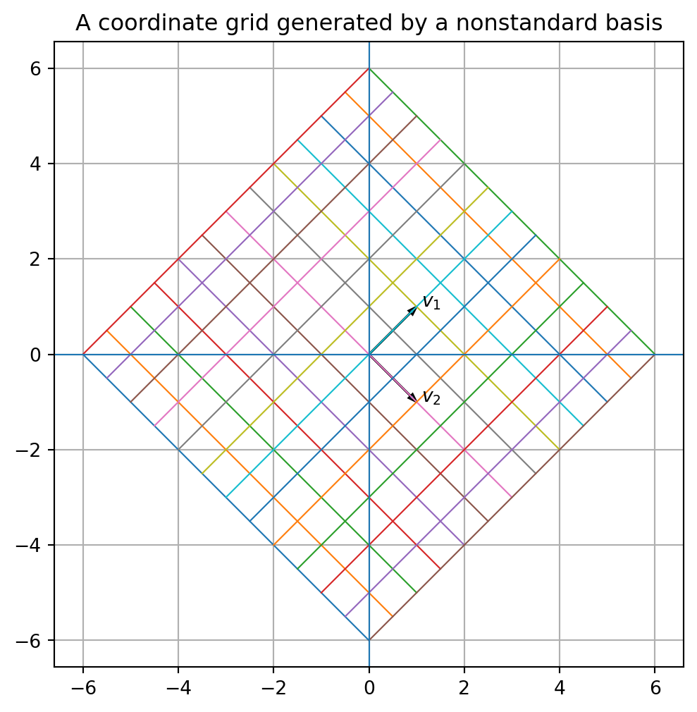
9.10 Coordinate grids
A basis creates a coordinate grid.
The standard basis creates square coordinate lines. A nonstandard basis creates a tilted or skewed grid.
The basis matrix maps the standard coordinate grid in coordinate space to the actual grid in vector space.
= np.array([[1 , 1 ],1 , - 1 ]], dtype= float )= np.linspace(- 3 , 3 , 13 )= (6 , 6 ))# Lines with fixed first coordinate for c1 in coeffs:= np.array([B @ np.array([c1, c2]) for c2 in coeffs])0 ], pts[:, 1 ], linewidth= 0.8 )# Lines with fixed second coordinate for c2 in coeffs:= np.array([B @ np.array([c1, c2]) for c1 in coeffs])0 ], pts[:, 1 ], linewidth= 0.8 )0 , 0 , B[0 ,0 ], B[1 ,0 ], head_width= 0.12 , length_includes_head= True )0 , 0 , B[0 ,1 ], B[1 ,1 ], head_width= 0.12 , length_includes_head= True )0 ,0 ]+ 0.1 , B[1 ,0 ], "$v_1$" )0 ,1 ]+ 0.1 , B[1 ,1 ], "$v_2$" )0 , linewidth= 0.8 )0 , linewidth= 0.8 )True )"equal" )"A coordinate grid generated by a nonstandard basis" )
9.11 Coordinates in a subspace
If \(W\) is a subspace of \(\mathbb{R}^n\) and
\[
\mathcal{B}=\{v_1,\ldots,v_p\}
\]
is a basis for \(W\) , then every vector \(w\in W\) has coordinates in \(\mathbb{R}^p\) relative to \(\mathcal{B}\) .
For example, a plane through the origin in \(\mathbb{R}^3\) may have basis
\[
v_1=
\begin{bmatrix}
1\\
0\\
1
\end{bmatrix},
\qquad
v_2=
\begin{bmatrix}
0\\
1\\
1
\end{bmatrix}.
\]
Then every vector in the plane can be written uniquely as
\[
w=c_1v_1+c_2v_2.
\]
Its coordinate vector relative to this basis is
\[
[w]_{\mathcal{B}}
=
\begin{bmatrix}
c_1\\
c_2
\end{bmatrix}.
\]
Notice that \(w\) lives in \(\mathbb{R}^3\) , but its coordinate vector relative to a basis of the plane lives in \(\mathbb{R}^2\) .
This is why dimension matters: coordinates use as many numbers as the dimension of the space, not necessarily the dimension of the ambient space.
9.12 Example: coordinates in a plane
Let
\[
W=\operatorname{span}
\left\{
v_1=
\begin{bmatrix}
1\\
0\\
1
\end{bmatrix},
\quad
v_2=
\begin{bmatrix}
0\\
1\\
1
\end{bmatrix}
\right\}.
\]
Let
\[
w=
\begin{bmatrix}
2\\
3\\
5
\end{bmatrix}.
\]
Since
\[
2v_1+3v_2
=
2
\begin{bmatrix}
1\\
0\\
1
\end{bmatrix}
+
3
\begin{bmatrix}
0\\
1\\
1
\end{bmatrix}
=
\begin{bmatrix}
2\\
3\\
5
\end{bmatrix},
\]
we have
\[
[w]_{\mathcal{B}}
=
\begin{bmatrix}
2\\
3
\end{bmatrix}.
\]
The vector \(w\) has three standard coordinates but only two coordinates relative to the plane basis.
9.14 Similarity preview
Two square matrices \(A\) and \(B\) are called similar if there is an invertible matrix \(P\) such that
\[
B=P^{-1}AP.
\]
Similar matrices represent the same linear transformation in different coordinate systems.
This idea will become central when we study eigenvectors and diagonalization.
If we can choose a basis made of eigenvectors, then the matrix of the transformation in that basis becomes diagonal:
\[
D=P^{-1}AP.
\]
Diagonalization is therefore a change of basis that reveals the simplest coordinate system for a transformation.
9.15 Why coordinates matter computationally
Choosing a good basis can make a problem simpler.
Examples:
A diagonal basis makes matrix powers easy.
An orthonormal basis makes projection easy.
A Fourier basis makes signals easier to analyze.
A principal component basis reveals dominant data directions.
A singular vector basis reveals the geometry of a matrix.
A sparse basis can compress information.
The same vector or transformation can look complicated in one basis and simple in another.
Much of linear algebra is the art of choosing the right coordinates.
9.16 Python: coordinates relative to a basis
import numpy as np= np.array([1 , 1 ],1 , - 1 ]= float )= np.array([3 , 1 ], dtype= float )= np.linalg.solve(P_B, b)
This returns
\[
[b]_{\mathcal{B}}
=
\begin{bmatrix}
2\\
1
\end{bmatrix}.
\]
To convert back to standard coordinates:
This returns the original vector \(b\) .
9.17 Python: change of basis between two bases
= np.array([1 , 1 ],1 , - 1 ]= float )= np.array([2 , 1 ],1 , 1 ]= float )= np.array([2 , 1 ], dtype= float )# Convert B-coordinates to standard coordinates = P_B @ x_B# Convert standard coordinates to C-coordinates = np.linalg.solve(P_C, x_standard)
(array([3., 1.]), array([ 2., -1.]))
The output gives
\[
x=
\begin{bmatrix}
3\\
1
\end{bmatrix},
\qquad
[x]_{\mathcal{C}}
=
\begin{bmatrix}
2\\
-1
\end{bmatrix}.
\]
The direct change-of-basis matrix from \(\mathcal{B}\) to \(\mathcal{C}\) is:
= np.linalg.solve(P_C, P_B)
array([[ 0.,  2.],
       [ 1., -3.]])
Then
gives the \(\mathcal{C}\) -coordinates directly.
9.18 Python: matrix representation in a new basis
Let
\[
A=
\begin{bmatrix}
2&1\\
0&3
\end{bmatrix}
\]
and
\[
P_{\mathcal{B}}=
\begin{bmatrix}
1&1\\
1&-1
\end{bmatrix}.
\]
The matrix of the same transformation in the \(\mathcal{B}\) basis is
\[
A_{\mathcal{B}}=P_{\mathcal{B}}^{-1}AP_{\mathcal{B}}.
\]
= np.array([2 , 1 ],0 , 3 ]= float )= np.array([1 , 1 ],1 , - 1 ]= float )= np.linalg.solve(P_B, A @ P_B)
array([[ 3., -1.],
       [-0.,  2.]])
This matrix tells how the transformation acts on \(\mathcal{B}\) -coordinates.
9.19 Python: comparing coordinate descriptions
= np.array([2 , 1 ], dtype= float )# Standard vector = P_B @ x_B# Apply A in standard coordinates = A @ x# Convert result to B-coordinates = np.linalg.solve(P_B, Ax_standard)# Apply A_B directly to B-coordinates = A_B @ x_B
(array([5., 2.]), array([5., 2.]))
The two answers are the same. This confirms that
\[
[T(x)]_{\mathcal{B}}=A_{\mathcal{B}}[x]_{\mathcal{B}}.
\]
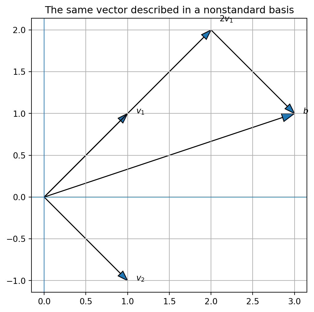
9.20 Python visualization: same vector, different coordinates
= np.array([1 , 1 ], dtype= float )= np.array([1 , - 1 ], dtype= float )= np.array([3 , 1 ], dtype= float )= (6 , 6 ))# basis vectors 0 , 0 , v1[0 ], v1[1 ], head_width= 0.08 , length_includes_head= True )0 , 0 , v2[0 ], v2[1 ], head_width= 0.08 , length_includes_head= True )# construction 2 v1 + 1 v2 0 , 0 , 2 * v1[0 ], 2 * v1[1 ], head_width= 0.08 , length_includes_head= True )2 * v1[0 ], 2 * v1[1 ], v2[0 ], v2[1 ], head_width= 0.08 , length_includes_head= True )# final vector 0 , 0 , b[0 ], b[1 ], head_width= 0.1 , length_includes_head= True )0 ]+ 0.1 , v1[1 ], "$v_1$" )0 ]+ 0.1 , v2[1 ], "$v_2$" )0 ]+ 0.1 , b[1 ], "$b$" )2.1 , 2.1 , "$2v_1$" )0 , linewidth= 0.8 )0 , linewidth= 0.8 )True )"equal" )"The same vector described in a nonstandard basis" )
9.21 Algorithmic summary
To find \([x]_{\mathcal{B}}\) :
Form the basis matrix
\[
P_{\mathcal{B}}=\begin{bmatrix}v_1&v_2&\cdots&v_n\end{bmatrix}.
\]
Solve
\[
P_{\mathcal{B}}c=x.
\]
The solution is
\[
[x]_{\mathcal{B}}=c.
\]
Compute
\[
x=P_{\mathcal{B}}[x]_{\mathcal{B}}.
\]
Compute
\[
[x]_{\mathcal{C}}
=
P_{\mathcal{C}}^{-1}P_{\mathcal{B}}[x]_{\mathcal{B}}.
\]
Equivalently, solve
\[
P_{\mathcal{C}}[x]_{\mathcal{C}}=P_{\mathcal{B}}[x]_{\mathcal{B}}.
\]
If \(A\) is the standard matrix and \(P_{\mathcal{B}}\) is a basis matrix, then
\[
A_{\mathcal{B}}=P_{\mathcal{B}}^{-1}AP_{\mathcal{B}}.
\]
9.22 Common mistakes
Mistake 1: confusing \(x\) with \([x]_{\mathcal{B}}\)
The vector \(x\) is the actual object in standard coordinates.
The vector \([x]_{\mathcal{B}}\) contains coefficients relative to the basis \(\mathcal{B}\) .
Mistake 2: putting basis vectors as rows
The basis matrix uses basis vectors as columns:
\[
P_{\mathcal{B}}=\begin{bmatrix}v_1&v_2&\cdots&v_n\end{bmatrix}.
\]
Mistake 3: using inverse when solve is better
Computationally, use
rather than
Mistake 4: reversing the direction of change of basis
The matrix
\[
P_{\mathcal{C}}^{-1}P_{\mathcal{B}}
\]
converts from \(\mathcal{B}\) -coordinates to \(\mathcal{C}\) -coordinates.
The reverse direction is
\[
P_{\mathcal{B}}^{-1}P_{\mathcal{C}}.
\]
9.23 Chapter summary
A basis gives a coordinate system.
If
\[
\mathcal{B}=\{v_1,\ldots,v_n\},
\]
then the basis matrix is
\[
P_{\mathcal{B}}=
\begin{bmatrix}
v_1&\cdots&v_n
\end{bmatrix}.
\]
Coordinates in the basis \(\mathcal{B}\) satisfy
\[
x=P_{\mathcal{B}}[x]_{\mathcal{B}}.
\]
Thus
\[
[x]_{\mathcal{B}}=P_{\mathcal{B}}^{-1}x.
\]
To change from \(\mathcal{B}\) -coordinates to \(\mathcal{C}\) -coordinates,
\[
[x]_{\mathcal{C}}
=
P_{\mathcal{C}}^{-1}P_{\mathcal{B}}[x]_{\mathcal{B}}.
\]
If \(A\) represents a linear transformation in standard coordinates, then its matrix in basis \(\mathcal{B}\) is
\[
A_{\mathcal{B}}=P_{\mathcal{B}}^{-1}AP_{\mathcal{B}}.
\]
This is the beginning of similarity and diagonalization.
Exercises
A. Coordinates in a basis
For each basis \(\mathcal{B}\) and vector \(x\) , find \([x]_{\mathcal{B}}\) .
\[
\mathcal{B}=
\left\{
\begin{bmatrix}1\\1\end{bmatrix},
\begin{bmatrix}1\\-1\end{bmatrix}
\right\},
\qquad
x=
\begin{bmatrix}3\\1\end{bmatrix}.
\]
\[
\mathcal{B}=
\left\{
\begin{bmatrix}2\\1\end{bmatrix},
\begin{bmatrix}1\\1\end{bmatrix}
\right\},
\qquad
x=
\begin{bmatrix}3\\1\end{bmatrix}.
\]
\[
\mathcal{B}=
\left\{
\begin{bmatrix}1\\0\\1\end{bmatrix},
\begin{bmatrix}0\\1\\1\end{bmatrix},
\begin{bmatrix}1\\1\\0\end{bmatrix}
\right\},
\qquad
x=
\begin{bmatrix}2\\3\\5\end{bmatrix}.
\]
B. From basis coordinates to standard coordinates
Compute \(x=P_{\mathcal{B}}[x]_{\mathcal{B}}\) .
\[
\mathcal{B}=
\left\{
\begin{bmatrix}1\\1\end{bmatrix},
\begin{bmatrix}1\\-1\end{bmatrix}
\right\},
\qquad
[x]_{\mathcal{B}}=
\begin{bmatrix}2\\1\end{bmatrix}.
\]
\[
\mathcal{B}=
\left\{
\begin{bmatrix}2\\1\end{bmatrix},
\begin{bmatrix}1\\1\end{bmatrix}
\right\},
\qquad
[x]_{\mathcal{B}}=
\begin{bmatrix}2\\-1\end{bmatrix}.
\]
\[
\mathcal{B}=
\left\{
\begin{bmatrix}1\\0\\1\end{bmatrix},
\begin{bmatrix}0\\1\\1\end{bmatrix}
\right\},
\qquad
[x]_{\mathcal{B}}=
\begin{bmatrix}2\\3\end{bmatrix}.
\]
C. Change of basis
Let
\[
\mathcal{B}=
\left\{
\begin{bmatrix}1\\1\end{bmatrix},
\begin{bmatrix}1\\-1\end{bmatrix}
\right\}
\]
and
\[
\mathcal{C}=
\left\{
\begin{bmatrix}2\\1\end{bmatrix},
\begin{bmatrix}1\\1\end{bmatrix}
\right\}.
\]
Find \(P_{\mathcal{B}}\) and \(P_{\mathcal{C}}\) .
Compute \(P_{\mathcal{C}\leftarrow\mathcal{B}}=P_{\mathcal{C}}^{-1}P_{\mathcal{B}}\) .
Use it to convert
\[
[x]_{\mathcal{B}}=
\begin{bmatrix}2\\1\end{bmatrix}
\]
to \(\mathcal{C}\) -coordinates. 4. Convert the result back to \(\mathcal{B}\) -coordinates.
D. Matrix representation in a new basis
Let
\[
A=
\begin{bmatrix}
2&1\\
0&3
\end{bmatrix}
\]
and
\[
\mathcal{B}=
\left\{
\begin{bmatrix}1\\1\end{bmatrix},
\begin{bmatrix}1\\-1\end{bmatrix}
\right\}.
\]
Form \(P_{\mathcal{B}}\) .
Compute
\[
A_{\mathcal{B}}=P_{\mathcal{B}}^{-1}AP_{\mathcal{B}}.
\]
Choose a vector \([x]_{\mathcal{B}}\) and verify that
\[
[T(x)]_{\mathcal{B}}=A_{\mathcal{B}}[x]_{\mathcal{B}}.
\]
E. Conceptual questions
What is the difference between a vector and its coordinates?
Why must a basis matrix be invertible?
What does \(P_{\mathcal{B}}[x]_{\mathcal{B}}\) compute?
What does \(P_{\mathcal{B}}^{-1}x\) compute?
Why does a change of basis matrix depend on two bases?
Why are similar matrices viewed as the same transformation in different coordinates?
F. Python exercises
Use NumPy to compute \([x]_{\mathcal{B}}\) for
\[
x=
\begin{bmatrix}3\\1\end{bmatrix},
\qquad
\mathcal{B}=
\left\{
\begin{bmatrix}1\\1\end{bmatrix},
\begin{bmatrix}1\\-1\end{bmatrix}
\right\}.
\]
Convert the coordinates back to standard coordinates.
Compute the change-of-basis matrix from
\[
\mathcal{B}=
\left\{
\begin{bmatrix}1\\1\end{bmatrix},
\begin{bmatrix}1\\-1\end{bmatrix}
\right\}
\]
to
\[
\mathcal{C}=
\left\{
\begin{bmatrix}2\\1\end{bmatrix},
\begin{bmatrix}1\\1\end{bmatrix}
\right\}.
\]
Plot the coordinate grid generated by the basis \(\mathcal{B}\) .
For
\[
A=
\begin{bmatrix}
2&1\\
0&3
\end{bmatrix},
\]
compute \(A_{\mathcal{B}}=P_{\mathcal{B}}^{-1}AP_{\mathcal{B}}\) .
G. Reflection
Write a short paragraph answering each question.
Why are coordinates not intrinsic to a vector?
Why can changing basis simplify a problem?
How does a basis act like a language for describing vectors?
Why is diagonalization a change-of-basis idea?
How do coordinate systems appear in data analysis?
AI-age connection
Changing basis is one of the most important ideas behind modern data analysis. A data set may look complicated in its original coordinates, but a better coordinate system can reveal structure. Principal component analysis chooses new axes aligned with dominant variation. Fourier methods choose coordinates based on waves. The SVD chooses input and output coordinates that reveal stretching directions of a matrix. In AI, representation learning can be viewed as the search for useful coordinates in high-dimensional spaces.