19  Eigenvalues and Eigenvectors

19.1 Opening question

Most vectors change direction when a matrix acts on them.

For example, if

\[ A= \begin{bmatrix} 2&1\\ 1&2 \end{bmatrix}, \]

then a typical vector \(x\) is transformed into a new vector \(Ax\) pointing in a different direction.

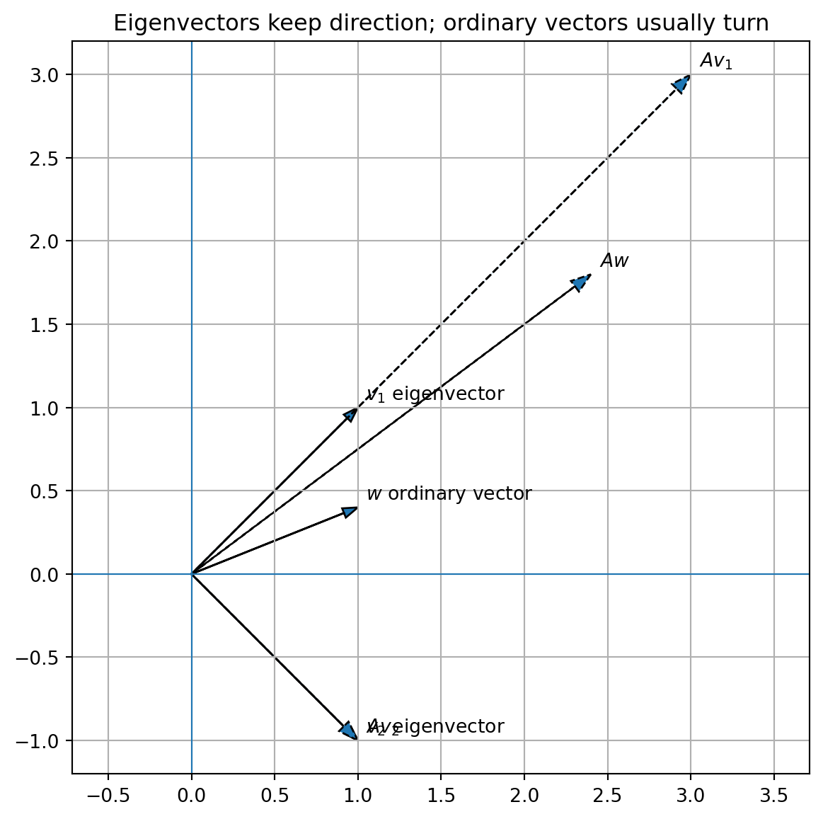
But some special vectors keep their direction. They are only stretched, compressed, or reversed.

These special vectors are eigenvectors.

If

\[ Ax=\lambda x, \]

then the matrix \(A\) acts on \(x\) in the simplest possible way: it only multiplies \(x\) by a scalar.

The scalar \(\lambda\) is the eigenvalue.

The central question of this chapter is:

Which directions does a matrix preserve?

Eigenvalues and eigenvectors reveal the natural directions of a linear transformation. They are essential for dynamical systems, diagonalization, Markov chains, stability, graph ranking, PCA, spectral clustering, and the SVD.

19.2 Learning goals

After studying this chapter, you should be able to:

  1. Define eigenvalues and eigenvectors.
  2. Check whether a vector is an eigenvector.
  3. Interpret eigenvectors geometrically.
  4. Derive the characteristic equation.
  5. Compute eigenvalues of \(2\times 2\) matrices.
  6. Find eigenspaces by solving homogeneous systems.
  7. Understand algebraic and geometric multiplicity.
  8. Recognize when a matrix may be diagonalizable.
  9. Use Python to compute and visualize eigenvectors.
  10. Connect eigenvalues to dynamics, stability, and data.

19.3 17.1 The eigenvector equation

Let \(A\) be an \(n\times n\) matrix.

A nonzero vector \(v\in\mathbb{R}^n\) is an eigenvector of \(A\) if there is a scalar \(\lambda\) such that

\[ Av=\lambda v. \]

The scalar \(\lambda\) is called the corresponding eigenvalue.

NoteDefinition: eigenvalue and eigenvector

For an \(n\times n\) matrix \(A\), a nonzero vector \(v\) is an eigenvector with eigenvalue \(\lambda\) if

\[ Av=\lambda v. \]

The vector \(v\) must be nonzero. The zero vector satisfies

\[ A0=\lambda 0 \]

for every \(\lambda\), so it is not allowed as an eigenvector.

19.4 17.2 Geometric meaning

The equation

\[ Av=\lambda v \]

means that \(Av\) lies on the same line as \(v\).

The matrix does not rotate \(v\) away from its own direction. It only scales that direction.

There are three common cases:

  • If \(\lambda>1\), the vector is stretched.
  • If \(0<\lambda<1\), the vector is compressed.
  • If \(\lambda<0\), the vector is reversed and scaled.
  • If \(\lambda=0\), the vector is collapsed to zero.

So an eigenvector is a direction preserved by the linear transformation.

19.5 17.3 First example

Let

\[ A= \begin{bmatrix} 3&0\\ 0&2 \end{bmatrix}. \]

Then

\[ A \begin{bmatrix} 1\\ 0 \end{bmatrix} = \begin{bmatrix} 3\\ 0 \end{bmatrix} = 3 \begin{bmatrix} 1\\ 0 \end{bmatrix}. \]

So

\[ e_1= \begin{bmatrix} 1\\ 0 \end{bmatrix} \]

is an eigenvector with eigenvalue \(3\).

Also,

\[ A \begin{bmatrix} 0\\ 1 \end{bmatrix} = \begin{bmatrix} 0\\ 2 \end{bmatrix} = 2 \begin{bmatrix} 0\\ 1 \end{bmatrix}. \]

So

\[ e_2= \begin{bmatrix} 0\\ 1 \end{bmatrix} \]

is an eigenvector with eigenvalue \(2\).

A diagonal matrix acts by scaling the coordinate axes.

19.6 17.4 Checking an eigenvector

Let

\[ A= \begin{bmatrix} 2&1\\ 1&2 \end{bmatrix}. \]

Check whether

\[ v_1= \begin{bmatrix} 1\\ 1 \end{bmatrix} \]

is an eigenvector.

Compute

\[ Av_1= \begin{bmatrix} 2&1\\ 1&2 \end{bmatrix} \begin{bmatrix} 1\\ 1 \end{bmatrix} = \begin{bmatrix} 3\\ 3 \end{bmatrix} = 3 \begin{bmatrix} 1\\ 1 \end{bmatrix}. \]

Therefore \(v_1\) is an eigenvector with eigenvalue

\[ \lambda=3. \]

Now check

\[ v_2= \begin{bmatrix} 1\\ -1 \end{bmatrix}. \]

Compute

\[ Av_2= \begin{bmatrix} 2&1\\ 1&2 \end{bmatrix} \begin{bmatrix} 1\\ -1 \end{bmatrix} = \begin{bmatrix} 1\\ -1 \end{bmatrix} = 1 \begin{bmatrix} 1\\ -1 \end{bmatrix}. \]

So \(v_2\) is an eigenvector with eigenvalue

\[ \lambda=1. \]

The matrix stretches the diagonal direction \([1,1]^T\) by \(3\) and leaves the anti-diagonal direction \([1,-1]^T\) unchanged.

19.7 17.5 Python plot: eigenvectors versus ordinary vectors

import numpy as np
import matplotlib.pyplot as plt

A = np.array([[2, 1],
              [1, 2]], dtype=float)

vectors = [
    (np.array([1, 1], dtype=float), "$v_1$ eigenvector"),
    (np.array([1, -1], dtype=float), "$v_2$ eigenvector"),
    (np.array([1, 0.4], dtype=float), "$w$ ordinary vector")
]

plt.figure(figsize=(7, 7))

for v, label in vectors:
    Av = A @ v
    plt.arrow(0, 0, v[0], v[1], head_width=0.06, length_includes_head=True)
    plt.arrow(0, 0, Av[0], Av[1], head_width=0.08, length_includes_head=True, linestyle="--")
    plt.text(v[0] + 0.05, v[1] + 0.05, label)
    plt.text(Av[0] + 0.05, Av[1] + 0.05, "$A$" + label.split()[0])

plt.axhline(0, linewidth=0.8)
plt.axvline(0, linewidth=0.8)
plt.grid(True)
plt.axis("equal")
plt.title("Eigenvectors keep direction; ordinary vectors usually turn")
plt.show()

19.8 17.6 From eigenvector equation to homogeneous system

The eigenvector equation is

\[ Av=\lambda v. \]

Move all terms to one side:

\[ Av-\lambda v=0. \]

Since

\[ \lambda v=\lambda Iv, \]

we get

\[ (A-\lambda I)v=0. \]

Thus \(v\) is an eigenvector if and only if it is a nonzero solution of

\[ (A-\lambda I)v=0. \]

This means \(A-\lambda I\) must have a nontrivial nullspace.

Therefore \(A-\lambda I\) must be singular.

So

\[ \det(A-\lambda I)=0. \]

This equation is the characteristic equation.

ImportantCharacteristic equation

The eigenvalues of \(A\) are the solutions of

\[ \det(A-\lambda I)=0. \]

19.9 17.7 Characteristic polynomial

The expression

\[ p_A(\lambda)=\det(A-\lambda I) \]

is called the characteristic polynomial of \(A\).

Some books use

\[ \det(\lambda I-A) \]

instead. The two forms differ by a sign when \(n\) is odd, but they have the same roots.

The roots of the characteristic polynomial are the eigenvalues.

19.10 17.8 Example: eigenvalues of a \(2\times 2\) matrix

Let

\[ A= \begin{bmatrix} 2&1\\ 1&2 \end{bmatrix}. \]

Compute

\[ A-\lambda I = \begin{bmatrix} 2-\lambda&1\\ 1&2-\lambda \end{bmatrix}. \]

Then

\[ \det(A-\lambda I) = (2-\lambda)^2-1. \]

Set this equal to zero:

\[ (2-\lambda)^2-1=0. \]

Factor:

\[ (2-\lambda-1)(2-\lambda+1)=0. \]

So

\[ (1-\lambda)(3-\lambda)=0. \]

Therefore

\[ \lambda=1 \]

or

\[ \lambda=3. \]

These match the eigenvalues we found by checking special vectors.

19.11 17.9 Finding eigenspaces

Once we know an eigenvalue \(\lambda\), the corresponding eigenvectors are the nonzero solutions of

\[ (A-\lambda I)v=0. \]

The solution set is the nullspace

\[ \operatorname{Null}(A-\lambda I). \]

This subspace is called the eigenspace for \(\lambda\).

NoteDefinition: eigenspace

The eigenspace of \(A\) corresponding to eigenvalue \(\lambda\) is

\[ E_\lambda=\operatorname{Null}(A-\lambda I). \]

The eigenspace contains the zero vector, but the eigenvectors are the nonzero vectors in that eigenspace.

19.12 17.10 Example: eigenspaces

Let

\[ A= \begin{bmatrix} 2&1\\ 1&2 \end{bmatrix}. \]

We found eigenvalues

\[ \lambda=3 \]

and

\[ \lambda=1. \]

19.12.1 Eigenspace for \(\lambda=3\)

Compute

\[ A-3I= \begin{bmatrix} -1&1\\ 1&-1 \end{bmatrix}. \]

Solve

\[ (A-3I)v=0. \]

This gives

\[ -x+y=0, \]

so

\[ y=x. \]

Thus

\[ E_3= \operatorname{span} \left\{ \begin{bmatrix} 1\\ 1 \end{bmatrix} \right\}. \]

19.12.2 Eigenspace for \(\lambda=1\)

Compute

\[ A-I= \begin{bmatrix} 1&1\\ 1&1 \end{bmatrix}. \]

Solve

\[ (A-I)v=0. \]

This gives

\[ x+y=0, \]

so

\[ y=-x. \]

Thus

\[ E_1= \operatorname{span} \left\{ \begin{bmatrix} 1\\ -1 \end{bmatrix} \right\}. \]

19.13 17.11 Python: eigenvalues and eigenvectors

import numpy as np

A = np.array([[2, 1],
              [1, 2]], dtype=float)

eigenvalues, eigenvectors = np.linalg.eig(A)

eigenvalues, eigenvectors
(array([3., 1.]),
 array([[ 0.70710678, -0.70710678],
        [ 0.70710678,  0.70710678]]))

The columns of eigenvectors are eigenvectors.

Check the eigenvector equation numerically:

for j in range(len(eigenvalues)):
    lam = eigenvalues[j]
    v = eigenvectors[:, j]
    print("lambda =", lam)
    print("A v =", A @ v)
    print("lambda v =", lam * v)
    print()
lambda = 3.0
A v = [2.12132034 2.12132034]
lambda v = [2.12132034 2.12132034]

lambda = 1.0
A v = [-0.70710678  0.70710678]
lambda v = [-0.70710678  0.70710678]

Because eigenvectors can be scaled, NumPy may return unit eigenvectors rather than the simple integer vectors.

19.14 17.12 Triangular matrices

Eigenvalues of triangular matrices are easy.

If \(A\) is upper triangular,

\[ A= \begin{bmatrix} a_{11}&*&\cdots&*\\ 0&a_{22}&\cdots&*\\ \vdots&\vdots&\ddots&\vdots\\ 0&0&\cdots&a_{nn} \end{bmatrix}, \]

then the eigenvalues are the diagonal entries:

\[ a_{11},a_{22},\ldots,a_{nn}. \]

Why?

The matrix

\[ A-\lambda I \]

is also upper triangular, with diagonal entries

\[ a_{11}-\lambda,\ldots,a_{nn}-\lambda. \]

Therefore

\[ \det(A-\lambda I) = (a_{11}-\lambda)\cdots(a_{nn}-\lambda). \]

So the roots are the diagonal entries.

ImportantEigenvalues of triangular matrices

The eigenvalues of a triangular matrix are its diagonal entries.

19.15 17.13 Example: triangular matrix

Let

\[ A= \begin{bmatrix} 4&2&1\\ 0&3&5\\ 0&0&-1 \end{bmatrix}. \]

Since \(A\) is upper triangular, its eigenvalues are

\[ 4,\quad 3,\quad -1. \]

No determinant expansion is needed.

19.16 17.14 Trace and determinant

For a \(2\times 2\) matrix

\[ A= \begin{bmatrix} a&b\\ c&d \end{bmatrix}, \]

the characteristic polynomial can be written as

\[ \lambda^2-\operatorname{tr}(A)\lambda+\det(A)=0, \]

where

\[ \operatorname{tr}(A)=a+d. \]

The trace is the sum of diagonal entries.

For a \(2\times 2\) matrix, the eigenvalues satisfy:

\[ \lambda_1+\lambda_2=\operatorname{tr}(A), \]

and

\[ \lambda_1\lambda_2=\det(A). \]

More generally, for an \(n\times n\) matrix, the determinant is the product of eigenvalues and the trace is the sum of eigenvalues, counted with multiplicity.

19.17 17.15 Complex eigenvalues

Some real matrices do not have real eigenvalues.

For example,

\[ R= \begin{bmatrix} 0&-1\\ 1&0 \end{bmatrix} \]

rotates the plane by \(90^\circ\).

Its characteristic equation is

\[ \det(R-\lambda I) = \det \begin{bmatrix} -\lambda&-1\\ 1&-\lambda \end{bmatrix} = \lambda^2+1=0. \]

Thus

\[ \lambda=\pm i. \]

There are no real eigenvalues.

Geometrically, this makes sense: a \(90^\circ\) rotation has no real direction that stays on the same line.

In this book, we will often focus on real eigenvalues and real eigenvectors, but complex eigenvalues are important in rotations, oscillations, and differential equations.

19.18 17.16 Eigenvalues and powers of a matrix

Eigenvectors make matrix powers easy.

If

\[ Av=\lambda v, \]

then

\[ A^2v=A(Av)=A(\lambda v)=\lambda Av=\lambda^2v. \]

Continuing,

\[ A^kv=\lambda^k v. \]

ImportantMatrix powers on eigenvectors

If \(Av=\lambda v\), then

\[ A^kv=\lambda^k v. \]

This is why eigenvalues are central in discrete dynamical systems.

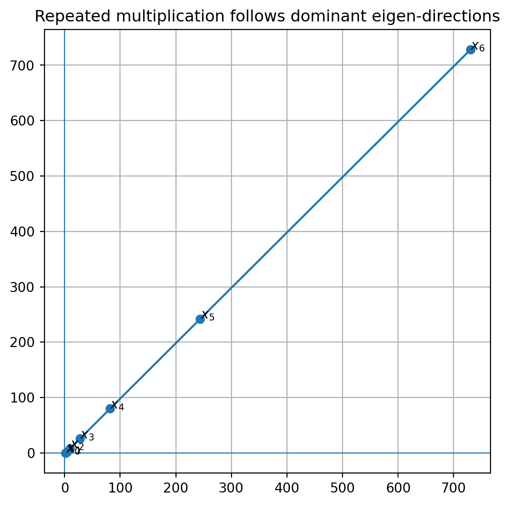
Repeated application of a matrix amplifies eigen-directions with large \(|\lambda|\) and suppresses eigen-directions with small \(|\lambda|\).

19.19 17.17 Dynamics example

Let

\[ A= \begin{bmatrix} 2&1\\ 1&2 \end{bmatrix}. \]

The eigenvectors are

\[ v_1= \begin{bmatrix} 1\\ 1 \end{bmatrix} \]

with eigenvalue \(3\), and

\[ v_2= \begin{bmatrix} 1\\ -1 \end{bmatrix} \]

with eigenvalue \(1\).

Suppose

\[ x_0= \begin{bmatrix} 2\\ 0 \end{bmatrix}. \]

We can write

\[ x_0=v_1+v_2. \]

Then

\[ A^kx_0 = A^k(v_1+v_2) = 3^kv_1+1^kv_2. \]

As \(k\) grows, the direction \(v_1\) dominates because \(3^k\) grows rapidly.

This is the basic idea behind many ranking and iteration algorithms.

19.20 17.18 Python plot: repeated multiplication

A = np.array([[2, 1],
              [1, 2]], dtype=float)

x = np.array([2, 0], dtype=float)
points = [x]

for k in range(6):
    x = A @ x
    points.append(x)

points = np.array(points)

plt.figure(figsize=(6, 6))
plt.plot(points[:, 0], points[:, 1], marker="o")
for k, p in enumerate(points):
    plt.text(p[0] + 0.1, p[1] + 0.1, f"$x_{k}$")

plt.axhline(0, linewidth=0.8)
plt.axvline(0, linewidth=0.8)
plt.grid(True)
plt.axis("equal")
plt.title("Repeated multiplication follows dominant eigen-directions")
plt.show()

19.21 17.19 Algebraic and geometric multiplicity

An eigenvalue may appear more than once as a root of the characteristic polynomial.

The number of times it appears is the algebraic multiplicity.

The dimension of its eigenspace is the geometric multiplicity.

NoteMultiplicity

For an eigenvalue \(\lambda\):

  • its algebraic multiplicity is its multiplicity as a root of the characteristic polynomial,
  • its geometric multiplicity is

\[ \dim(E_\lambda). \]

Always,

\[ 1\le \text{geometric multiplicity}\le \text{algebraic multiplicity}. \]

19.22 17.20 Example: repeated eigenvalue with enough eigenvectors

Let

\[ A= \begin{bmatrix} 2&0\\ 0&2 \end{bmatrix} = 2I. \]

The only eigenvalue is

\[ \lambda=2 \]

with algebraic multiplicity \(2\).

But

\[ A-2I=0, \]

so

\[ E_2=\mathbb{R}^2. \]

Thus the geometric multiplicity is \(2\).

Every nonzero vector is an eigenvector.

19.23 17.21 Example: repeated eigenvalue without enough eigenvectors

Let

\[ A= \begin{bmatrix} 2&1\\ 0&2 \end{bmatrix}. \]

The characteristic polynomial is

\[ (2-\lambda)^2. \]

So

\[ \lambda=2 \]

has algebraic multiplicity \(2\).

Now compute

\[ A-2I= \begin{bmatrix} 0&1\\ 0&0 \end{bmatrix}. \]

Solving

\[ (A-2I)v=0 \]

gives

\[ y=0. \]

So

\[ E_2= \operatorname{span} \left\{ \begin{bmatrix} 1\\ 0 \end{bmatrix} \right\}. \]

The eigenspace has dimension \(1\).

Thus the geometric multiplicity is \(1\), less than the algebraic multiplicity.

This matrix does not have enough eigenvectors to form a basis of \(\mathbb{R}^2\).

19.24 17.22 Eigenvectors with distinct eigenvalues are independent

ImportantIndependence theorem

Eigenvectors corresponding to distinct eigenvalues are linearly independent.

For example, if a \(2\times 2\) matrix has two distinct real eigenvalues, then its two eigenvectors are automatically linearly independent.

If a \(3\times 3\) matrix has three distinct real eigenvalues, then its three eigenvectors are automatically linearly independent.

This theorem is the foundation of diagonalization.

19.25 17.23 Diagonalization preview

If an \(n\times n\) matrix \(A\) has \(n\) linearly independent eigenvectors

\[ v_1,\ldots,v_n \]

with eigenvalues

\[ \lambda_1,\ldots,\lambda_n, \]

then form

\[ P= \begin{bmatrix} v_1&v_2&\cdots&v_n \end{bmatrix} \]

and

\[ D= \begin{bmatrix} \lambda_1&0&\cdots&0\\ 0&\lambda_2&\cdots&0\\ \vdots&\vdots&\ddots&\vdots\\ 0&0&\cdots&\lambda_n \end{bmatrix}. \]

Then

\[ AP=PD. \]

If \(P\) is invertible, then

\[ A=PDP^{-1}. \]

Equivalently,

\[ P^{-1}AP=D. \]

This means that \(A\) becomes diagonal in an eigenvector basis.

Diagonalization will be studied in detail in the next chapter.

19.26 17.24 Python: diagonalization preview

A = np.array([[2, 1],
              [1, 2]], dtype=float)

eigvals, P = np.linalg.eig(A)

D = np.diag(eigvals)

P_inv_A_P = np.linalg.inv(P) @ A @ P

D, P_inv_A_P
(array([[3., 0.],
        [0., 1.]]),
 array([[3., 0.],
        [0., 1.]]))

The output shows that, up to numerical roundoff,

\[ P^{-1}AP=D. \]

19.27 17.25 Symmetric matrices preview

The matrix

\[ A= \begin{bmatrix} 2&1\\ 1&2 \end{bmatrix} \]

is symmetric because

\[ A^T=A. \]

Symmetric matrices have especially beautiful eigenvalue behavior:

  • all eigenvalues are real,
  • eigenvectors for distinct eigenvalues are orthogonal,
  • there is an orthonormal basis of eigenvectors.

These facts lead to the spectral theorem.

We will study them later.

19.28 17.26 Markov chains and ranking preview

Eigenvectors also appear in systems that evolve by repeated multiplication.

If

\[ x_{k+1}=Ax_k, \]

then long-term behavior is controlled by eigenvalues and eigenvectors.

In ranking algorithms, a dominant eigenvector can represent a steady-state importance score.

In Markov chains, an eigenvector associated with eigenvalue \(1\) can represent a stationary distribution.

In stability analysis, eigenvalues tell whether repeated iteration grows or decays.

19.29 17.27 Python: dominant eigenvector iteration

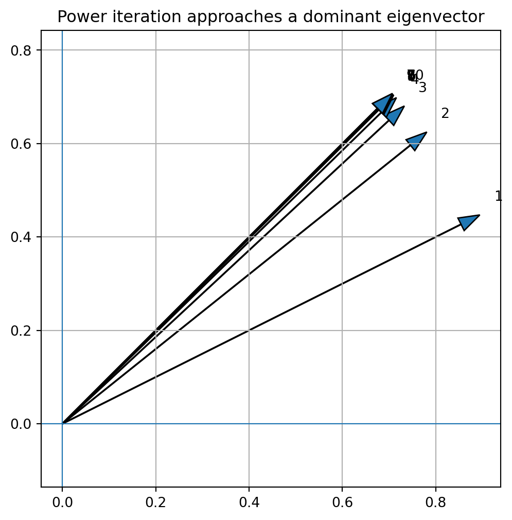
Power iteration is a simple algorithm for approximating a dominant eigenvector.

A = np.array([[2, 1],
              [1, 2]], dtype=float)

x = np.array([1, 0], dtype=float)

history = []

for k in range(10):
    x = A @ x
    x = x / np.linalg.norm(x)
    history.append(x.copy())

np.array(history)
array([[0.89442719, 0.4472136 ],
       [0.78086881, 0.62469505],
       [0.73279349, 0.6804511 ],
       [0.71578195, 0.69832385],
       [0.71001067, 0.70419091],
       [0.70807608, 0.70613615],
       [0.70743003, 0.70678338],
       [0.70721455, 0.706999  ],
       [0.70714271, 0.70707086],
       [0.70711876, 0.70709481]])

The vectors approach the dominant eigenvector direction.

history = np.array(history)

plt.figure(figsize=(6, 6))
for k, v in enumerate(history):
    plt.arrow(0, 0, v[0], v[1], head_width=0.03, length_includes_head=True)
    plt.text(v[0] + 0.03, v[1] + 0.03, str(k+1))

plt.axhline(0, linewidth=0.8)
plt.axvline(0, linewidth=0.8)
plt.grid(True)
plt.axis("equal")
plt.title("Power iteration approaches a dominant eigenvector")
plt.show()

19.30 17.28 Algorithmic summary

NoteAlgorithm: check an eigenpair

To check whether \((\lambda,v)\) is an eigenpair:

  1. Verify that \(v\ne 0\).
  2. Compute \(Av\).
  3. Compute \(\lambda v\).
  4. Check whether

\[ Av=\lambda v. \]

NoteAlgorithm: find eigenvalues

To find eigenvalues of a square matrix \(A\):

  1. Form

\[ A-\lambda I. \]

  1. Compute

\[ \det(A-\lambda I). \]

  1. Solve

\[ \det(A-\lambda I)=0. \]

NoteAlgorithm: find eigenvectors

For each eigenvalue \(\lambda\):

  1. Form

\[ A-\lambda I. \]

  1. Solve

\[ (A-\lambda I)v=0. \]

  1. The nonzero solutions are eigenvectors.
  2. The full solution space is the eigenspace \(E_\lambda\).
NoteAlgorithm: dominant eigenvector by power iteration

Given a matrix \(A\) and a starting vector \(x_0\):

  1. Compute \(y_k=Ax_k\).
  2. Normalize

\[ x_{k+1}=\frac{y_k}{\|y_k\|}. \]

  1. Repeat until the direction stabilizes.

19.31 17.29 Common mistakes

19.31.1 Mistake 1: allowing the zero vector as an eigenvector

The zero vector is never an eigenvector.

19.31.2 Mistake 2: confusing eigenvalues and eigenvectors

An eigenvalue is a scalar.

An eigenvector is a nonzero vector.

19.31.3 Mistake 3: solving \(\det(A)=0\) instead of \(\det(A-\lambda I)=0\)

Eigenvalues come from

\[ \det(A-\lambda I)=0. \]

19.31.4 Mistake 4: forgetting to find eigenspaces

Finding eigenvalues is only the first step. For each eigenvalue, solve

\[ (A-\lambda I)v=0. \]

19.31.5 Mistake 5: assuming every matrix has real eigenvalues

Real matrices can have complex eigenvalues.

A \(90^\circ\) rotation has eigenvalues \(\pm i\).

19.31.6 Mistake 6: assuming repeated eigenvalues always give repeated eigenvectors

Algebraic multiplicity and geometric multiplicity can differ.

19.32 17.30 Chapter summary

An eigenvector of a square matrix \(A\) is a nonzero vector \(v\) satisfying

\[ Av=\lambda v. \]

The scalar \(\lambda\) is the eigenvalue.

Eigenvectors are directions preserved by the transformation.

Eigenvalues are found from the characteristic equation

\[ \det(A-\lambda I)=0. \]

For an eigenvalue \(\lambda\), the eigenspace is

\[ E_\lambda=\operatorname{Null}(A-\lambda I). \]

Triangular matrices have eigenvalues equal to their diagonal entries.

For a \(2\times 2\) matrix, the sum of eigenvalues is the trace and the product is the determinant.

Eigenvectors corresponding to distinct eigenvalues are linearly independent.

If an \(n\times n\) matrix has \(n\) independent eigenvectors, then it can be diagonalized.

Eigenvalues control powers of matrices, dynamical systems, stability, ranking, and many algorithms in data science and AI.

19.33 Exercises

19.33.1 A. Checking eigenvectors

For each matrix and vector, determine whether the vector is an eigenvector. If so, find the eigenvalue.

\[ A= \begin{bmatrix} 3&0\\ 0&2 \end{bmatrix}, \qquad v= \begin{bmatrix} 1\\ 0 \end{bmatrix}. \]

\[ A= \begin{bmatrix} 2&1\\ 1&2 \end{bmatrix}, \qquad v= \begin{bmatrix} 1\\ 1 \end{bmatrix}. \]

\[ A= \begin{bmatrix} 2&1\\ 1&2 \end{bmatrix}, \qquad v= \begin{bmatrix} 1\\ 0 \end{bmatrix}. \]

\[ A= \begin{bmatrix} 1&2\\ 0&3 \end{bmatrix}, \qquad v= \begin{bmatrix} 1\\ 1 \end{bmatrix}. \]

19.33.2 B. Eigenvalues of \(2\times 2\) matrices

Find the eigenvalues of each matrix.

\[ \begin{bmatrix} 2&1\\ 1&2 \end{bmatrix} \]

\[ \begin{bmatrix} 3&0\\ 0&2 \end{bmatrix} \]

\[ \begin{bmatrix} 1&2\\ 0&3 \end{bmatrix} \]

\[ \begin{bmatrix} 0&-1\\ 1&0 \end{bmatrix} \]

\[ \begin{bmatrix} 2&1\\ 0&2 \end{bmatrix} \]

19.33.3 C. Eigenspaces

For each matrix in Exercise B, find a basis for each real eigenspace.

19.33.4 D. Triangular matrices

Find the eigenvalues of each triangular matrix.

\[ \begin{bmatrix} 4&2&1\\ 0&3&5\\ 0&0&-1 \end{bmatrix} \]

\[ \begin{bmatrix} 1&0&0\\ 2&5&0\\ 3&4&-2 \end{bmatrix} \]

\[ \begin{bmatrix} 2&1&0\\ 0&2&1\\ 0&0&2 \end{bmatrix} \]

19.33.5 E. Trace and determinant

For each \(2\times 2\) matrix, compute trace, determinant, eigenvalues, and verify

\[ \lambda_1+\lambda_2=\operatorname{tr}(A), \]

and

\[ \lambda_1\lambda_2=\det(A). \]

\[ \begin{bmatrix} 2&1\\ 1&2 \end{bmatrix} \]

\[ \begin{bmatrix} 1&2\\ 0&3 \end{bmatrix} \]

\[ \begin{bmatrix} 4&1\\ 2&3 \end{bmatrix} \]

19.33.6 F. Dynamics

Let

\[ A= \begin{bmatrix} 2&1\\ 1&2 \end{bmatrix}. \]

  1. Find eigenvalues and eigenvectors.
  2. Write

\[ x_0= \begin{bmatrix} 2\\ 0 \end{bmatrix} \]

as a linear combination of eigenvectors. 3. Compute a formula for \(A^kx_0\). 4. Describe the dominant direction as \(k\) grows.

19.33.7 G. Python exercises

  1. Use NumPy to compute eigenvalues and eigenvectors of several \(2\times 2\) matrices.
  2. Use SymPy to compute exact characteristic polynomials.
  3. Plot eigenvectors and their images under a matrix.
  4. Use power iteration to approximate a dominant eigenvector.
  5. Test a rotation matrix and observe its complex eigenvalues.
  6. For a symmetric matrix, check that eigenvectors for distinct eigenvalues are orthogonal.

19.33.8 H. Reflection

Write a short paragraph answering each question.

  1. Why are eigenvectors natural directions of a matrix?
  2. Why does \(\det(A-\lambda I)=0\) find eigenvalues?
  3. What is the difference between an eigenvector and an eigenspace?
  4. Why do eigenvalues control repeated multiplication?
  5. Why are eigenvalues important in data science and AI?

19.34 AI-age connection

Eigenvalues and eigenvectors are central to modern computation. They explain stability in dynamical systems, long-term behavior in Markov chains, ranking in networks, modes of vibration, principal directions in data, and the geometry of symmetric matrices. Spectral methods in graph learning, PCA, matrix factorization, and many AI algorithms all begin with the idea that a matrix has special directions that reveal its structure.