Opening question
A matrix can represent a process:
\[
x \longmapsto Ax.
\]
Sometimes the process can be reversed. If we know the output \(b\) , we can recover the input \(x\) .
That means we can solve
\[
Ax=b
\]
by undoing the action of \(A\) .
This chapter studies when a matrix can be undone.
The key object is the inverse matrix .
The key computational method is Gauss–Jordan elimination on \([A\mid I]\) .
The key conceptual result is the Invertible Matrix Theorem , which connects many different ways of saying that a square matrix has no information loss.
Learning goals
After studying this chapter, you should be able to:
Define the inverse of a square matrix.
Determine whether a \(2\times 2\) matrix is invertible.
Compute the inverse of a \(2\times 2\) matrix using the formula.
Compute inverses using Gauss–Jordan elimination.
Understand why row operations can be represented by elementary matrices.
Use an inverse to solve \(Ax=b\) when \(A\) is invertible.
Recognize equivalent descriptions of invertibility.
Interpret invertibility geometrically as no collapse of dimension.
Understand why solving by inverse is usually not the best numerical method.
Use Python to compute inverses, solve systems, and visualize invertible and noninvertible transformations.
5.1 What does it mean to undo a matrix?
For ordinary numbers, if \(a\ne 0\) , then the inverse of \(a\) is \(\frac1a\) , and
\[
\frac1a a = 1.
\]
For matrices, the identity matrix \(I\) plays the role of the number \(1\) .
Let \(A\) be an \(n\times n\) matrix. An \(n\times n\) matrix \(A^{-1}\) is called the inverse of \(A\) if
\[
A^{-1}A=I_n
\]
and
\[
AA^{-1}=I_n.
\]
If such a matrix exists, then \(A\) is called invertible or nonsingular .
If no inverse exists, then \(A\) is called singular .
The inverse reverses the action of \(A\) .
If
\[
Ax=b,
\]
and \(A\) is invertible, then multiply both sides by \(A^{-1}\) :
\[
A^{-1}Ax=A^{-1}b.
\]
Since
\[
A^{-1}A=I,
\]
we get
\[
x=A^{-1}b.
\]
So when \(A\) is invertible, the system \(Ax=b\) has the unique solution
\[
x=A^{-1}b.
\]
5.2 A first example
Let
\[
A=
\begin{bmatrix}
2&0\\
0&3
\end{bmatrix}.
\]
This matrix scales the first coordinate by \(2\) and the second coordinate by \(3\) :
\[
A
\begin{bmatrix}
x\\
y
\end{bmatrix}
=
\begin{bmatrix}
2x\\
3y
\end{bmatrix}.
\]
To undo this transformation, divide the first coordinate by \(2\) and the second coordinate by \(3\) .
Thus
\[
A^{-1}=
\begin{bmatrix}
\frac12&0\\
0&\frac13
\end{bmatrix}.
\]
Check:
\[
A^{-1}A=
\begin{bmatrix}
\frac12&0\\
0&\frac13
\end{bmatrix}
\begin{bmatrix}
2&0\\
0&3
\end{bmatrix}
=
\begin{bmatrix}
1&0\\
0&1
\end{bmatrix}
=I_2.
\]
Also,
\[
AA^{-1}=I_2.
\]
5.3 The inverse of a \(2\times 2\) matrix
For a \(2\times 2\) matrix
\[
A=
\begin{bmatrix}
a&b\\
c&d
\end{bmatrix},
\]
the determinant is
\[
\det(A)=ad-bc.
\]
If
\[
ad-bc\ne 0,
\]
then \(A\) is invertible and
\[
A^{-1}
=
\frac{1}{ad-bc}
\begin{bmatrix}
d&-b\\
-c&a
\end{bmatrix}.
\]
If
\[
ad-bc=0,
\]
then \(A\) is not invertible.
\[
\begin{bmatrix}
a&b\\
c&d
\end{bmatrix}^{-1}
=
\frac{1}{ad-bc}
\begin{bmatrix}
d&-b\\
-c&a
\end{bmatrix},
\qquad ad-bc\ne 0.
\]
5.5 Example of a noninvertible matrix
Let
\[
A=
\begin{bmatrix}
1&2\\
2&4
\end{bmatrix}.
\]
Then
\[
\det(A)=1(4)-2(2)=0.
\]
So \(A\) is not invertible.
Why geometrically?
The second column is twice the first column:
\[
\begin{bmatrix}
2\\
4
\end{bmatrix}
=
2
\begin{bmatrix}
1\\
2
\end{bmatrix}.
\]
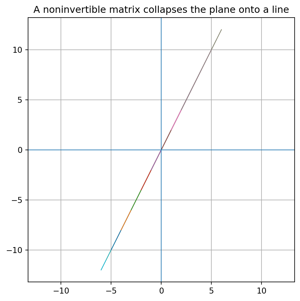
Therefore the two columns point in the same direction. The matrix cannot produce all vectors in \(\mathbb{R}^2\) . It collapses the plane onto a line.
Once a two-dimensional plane is collapsed onto a one-dimensional line, information is lost. We cannot reverse the process.
5.6 Geometry of invertibility in \(\mathbb{R}^2\)
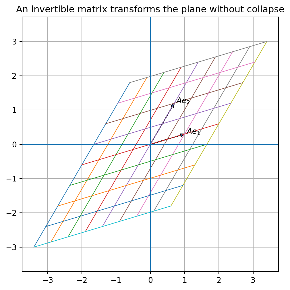
A \(2\times 2\) matrix transforms the plane.
If the matrix is invertible, it sends the plane to the whole plane. It may rotate, reflect, shear, stretch, or shrink, but it does not collapse area to zero.
If the matrix is not invertible, it collapses the plane into a line or a point.
5.7 Computing inverses by Gauss–Jordan elimination
The \(2\times 2\) formula is useful, but it does not scale well to large matrices.
For general \(n\times n\) matrices, we compute inverses using row reduction.
The idea is:
\[
[A\mid I] \longrightarrow [I\mid A^{-1}].
\]
If row reduction turns the left side into \(I\) , then the right side becomes \(A^{-1}\) .
If the left side cannot be turned into \(I\) , then \(A\) is not invertible.
To find \(A^{-1}\) :
Form the augmented matrix \([A\mid I_n]\) .
Use Gauss–Jordan elimination.
If the left side becomes \(I_n\) , then the right side is \(A^{-1}\) .
If the left side does not become \(I_n\) , then \(A\) is not invertible.
5.8 Example: inverse by row reduction
Let
\[
A=
\begin{bmatrix}
1&1&1\\
1&2&3\\
1&3&6
\end{bmatrix}.
\]
Start with
\[
[A\mid I]
=
\left[
\begin{array}{ccc|ccc}
1&1&1&1&0&0\\
1&2&3&0&1&0\\
1&3&6&0&0&1
\end{array}
\right].
\]
Apply row operations.
First eliminate below the first pivot:
\[
R_2\leftarrow R_2-R_1,
\qquad
R_3\leftarrow R_3-R_1.
\]
Then
\[
\left[
\begin{array}{ccc|ccc}
1&1&1&1&0&0\\
0&1&2&-1&1&0\\
0&2&5&-1&0&1
\end{array}
\right].
\]
Eliminate below the second pivot:
\[
R_3\leftarrow R_3-2R_2.
\]
Then
\[
\left[
\begin{array}{ccc|ccc}
1&1&1&1&0&0\\
0&1&2&-1&1&0\\
0&0&1&1&-2&1
\end{array}
\right].
\]
Eliminate above the third pivot:
\[
R_2\leftarrow R_2-2R_3,
\qquad
R_1\leftarrow R_1-R_3.
\]
Then
\[
\left[
\begin{array}{ccc|ccc}
1&1&0&0&2&-1\\
0&1&0&-3&5&-2\\
0&0&1&1&-2&1
\end{array}
\right].
\]
Eliminate above the second pivot:
\[
R_1\leftarrow R_1-R_2.
\]
Then
\[
\left[
\begin{array}{ccc|ccc}
1&0&0&3&-3&1\\
0&1&0&-3&5&-2\\
0&0&1&1&-2&1
\end{array}
\right].
\]
Therefore
\[
A^{-1}
=
\begin{bmatrix}
3&-3&1\\
-3&5&-2\\
1&-2&1
\end{bmatrix}.
\]
5.9 Checking an inverse
We should always check an inverse by multiplication.
For
\[
A=
\begin{bmatrix}
1&1&1\\
1&2&3\\
1&3&6
\end{bmatrix}
\]
and
\[
B=
\begin{bmatrix}
3&-3&1\\
-3&5&-2\\
1&-2&1
\end{bmatrix},
\]
we compute
\[
AB=I_3
\]
and
\[
BA=I_3.
\]
In practice, for square matrices, if one of these identities holds exactly, then the other also holds. But when learning, it is useful to understand that the definition of inverse requires both.
5.10 Solving systems using an inverse
Suppose
\[
Ax=b,
\]
where
\[
A=
\begin{bmatrix}
1&1&1\\
1&2&3\\
1&3&6
\end{bmatrix}
\]
and
\[
b=
\begin{bmatrix}
3\\
5\\
8
\end{bmatrix}.
\]
Since
\[
A^{-1}
=
\begin{bmatrix}
3&-3&1\\
-3&5&-2\\
1&-2&1
\end{bmatrix},
\]
we get
\[
x=A^{-1}b.
\]
Compute:
\[
x=
\begin{bmatrix}
3&-3&1\\
-3&5&-2\\
1&-2&1
\end{bmatrix}
\begin{bmatrix}
3\\
5\\
8
\end{bmatrix}
=
\begin{bmatrix}
2\\
-2\\
3
\end{bmatrix}.
\]
Thus the solution is
\[
x_1=2,\qquad x_2=-2,\qquad x_3=3.
\]
5.11 Elementary matrices
Every elementary row operation can be performed by multiplying on the left by a special matrix called an elementary matrix .
An elementary matrix is obtained by applying one elementary row operation to an identity matrix.
For example, start with
\[
I_3=
\begin{bmatrix}
1&0&0\\
0&1&0\\
0&0&1
\end{bmatrix}.
\]
If we swap rows \(1\) and \(2\) , we get the elementary matrix
\[
E=
\begin{bmatrix}
0&1&0\\
1&0&0\\
0&0&1
\end{bmatrix}.
\]
Multiplying \(EA\) swaps rows \(1\) and \(2\) of \(A\) .
If we multiply row \(2\) of \(I_3\) by \(5\) , we get
\[
E=
\begin{bmatrix}
1&0&0\\
0&5&0\\
0&0&1
\end{bmatrix}.
\]
Multiplying \(EA\) multiplies row \(2\) of \(A\) by \(5\) .
If we add \(3\) times row \(1\) to row \(3\) of \(I_3\) , we get
\[
E=
\begin{bmatrix}
1&0&0\\
0&1&0\\
3&0&1
\end{bmatrix}.
\]
Multiplying \(EA\) replaces row \(3\) of \(A\) by row \(3\) plus \(3\) times row \(1\) .
5.12 Why elementary matrices matter
Suppose row reduction turns \(A\) into \(I\) .
Each row operation is multiplication by an elementary matrix. So there are elementary matrices \(E_1,E_2,\ldots,E_k\) such that
\[
E_k\cdots E_2E_1A=I.
\]
This means
\[
E_k\cdots E_2E_1=A^{-1}.
\]
When we row reduce
\[
[A\mid I],
\]
the same row operations are applied to both sides:
\[
[E_k\cdots E_1A\mid E_k\cdots E_1I].
\]
If the left side becomes \(I\) , the right side becomes
\[
E_k\cdots E_1I=A^{-1}.
\]
This explains why the algorithm works.
5.13 The Invertible Matrix Theorem
The following theorem is one of the central organizing results of first linear algebra.
Let \(A\) be an \(n\times n\) matrix. The following statements are equivalent:
\(A\) is invertible.\(Ax=b\) has a unique solution for every \(b\in\mathbb{R}^n\) .\(Ax=0\) has only the trivial solution \(x=0\) .The reduced row-echelon form of \(A\) is \(I_n\) .
\(A\) has a pivot in every column.\(A\) has a pivot in every row.The columns of \(A\) span \(\mathbb{R}^n\) .
The columns of \(A\) are linearly independent.
The linear transformation \(x\mapsto Ax\) is one-to-one.
The linear transformation \(x\mapsto Ax\) maps \(\mathbb{R}^n\) onto \(\mathbb{R}^n\) .
\(\det(A)\ne 0\) .
Some of these ideas will be developed more deeply in later chapters. For now, the theorem gives a map of the subject.
Invertibility means all of these things at once:
no lost information,
no collapsed dimension,
unique solvability,
full set of pivots,
independent columns,
spanning columns,
nonzero determinant.
5.14 Invertibility and homogeneous systems
A square matrix \(A\) is invertible if and only if the homogeneous system
\[
Ax=0
\]
has only the zero solution.
Why?
If \(A\) is invertible and \(Ax=0\) , then multiply by \(A^{-1}\) :
\[
A^{-1}Ax=A^{-1}0.
\]
So
\[
x=0.
\]
Thus no nonzero vector can be sent to zero.
Geometrically, this means an invertible transformation does not collapse any nonzero direction to the origin.
If a nonzero vector \(v\) satisfies
\[
Av=0,
\]
then information is lost. The transformation cannot be invertible.
5.15 Invertibility and columns
Let
\[
A=
\begin{bmatrix}
|&|&&|\\
a_1&a_2&\cdots&a_n\\
|&|&&|
\end{bmatrix}.
\]
The equation
\[
Ax=b
\]
means
\[
x_1a_1+x_2a_2+\cdots+x_na_n=b.
\]
If \(A\) is invertible, then every \(b\in\mathbb{R}^n\) can be written in exactly one way as a linear combination of the columns of \(A\) .
So the columns of \(A\) must:
span \(\mathbb{R}^n\) ,
be linearly independent.
This means the columns form a basis of \(\mathbb{R}^n\) .
This will become a central idea in the chapters on span, linear independence, basis, and dimension.
5.17 Numerical warning: inverse versus solve
Although the formula
\[
x=A^{-1}b
\]
is mathematically correct, it is usually not the best way to solve a system on a computer.
In numerical computation, it is better to use a direct solver such as
rather than explicitly computing
The direct solver is usually faster and more accurate.
Use inverses for theory.
Use solvers for computation.
5.18 Python: computing an inverse
import numpy as np= np.array([1 , 1 , 1 ],1 , 2 , 3 ],1 , 3 , 6 ]= float )= np.linalg.inv(A)
array([[ 3., -3.,  1.],
       [-3.,  5., -2.],
       [ 1., -2.,  1.]])
Check:
array([[1., 0., 0.],
       [0., 1., 0.],
       [0., 0., 1.]])
Because of floating-point arithmetic, the result may contain tiny roundoff errors such as \(10^{-16}\) instead of exact zeros.
5.19 Python: solving with inverse versus solve
= np.array([3 , 5 , 8 ], dtype= float )= np.linalg.inv(A) @ b= np.linalg.solve(A, b)
(array([2., 0., 1.]), array([2., 0., 1.]))
Both should give approximately
\[
\begin{bmatrix}
2\\
-2\\
3
\end{bmatrix}.
\]
The second method is preferred computationally.
5.20 Python: a singular matrix
= np.array([1 , 2 ],2 , 4 ]= float )
The determinant is zero, so the matrix is singular.
Trying to invert it gives an error:
# Uncomment to see the error:
# np.linalg.inv(S)
5.21 Condition number preview
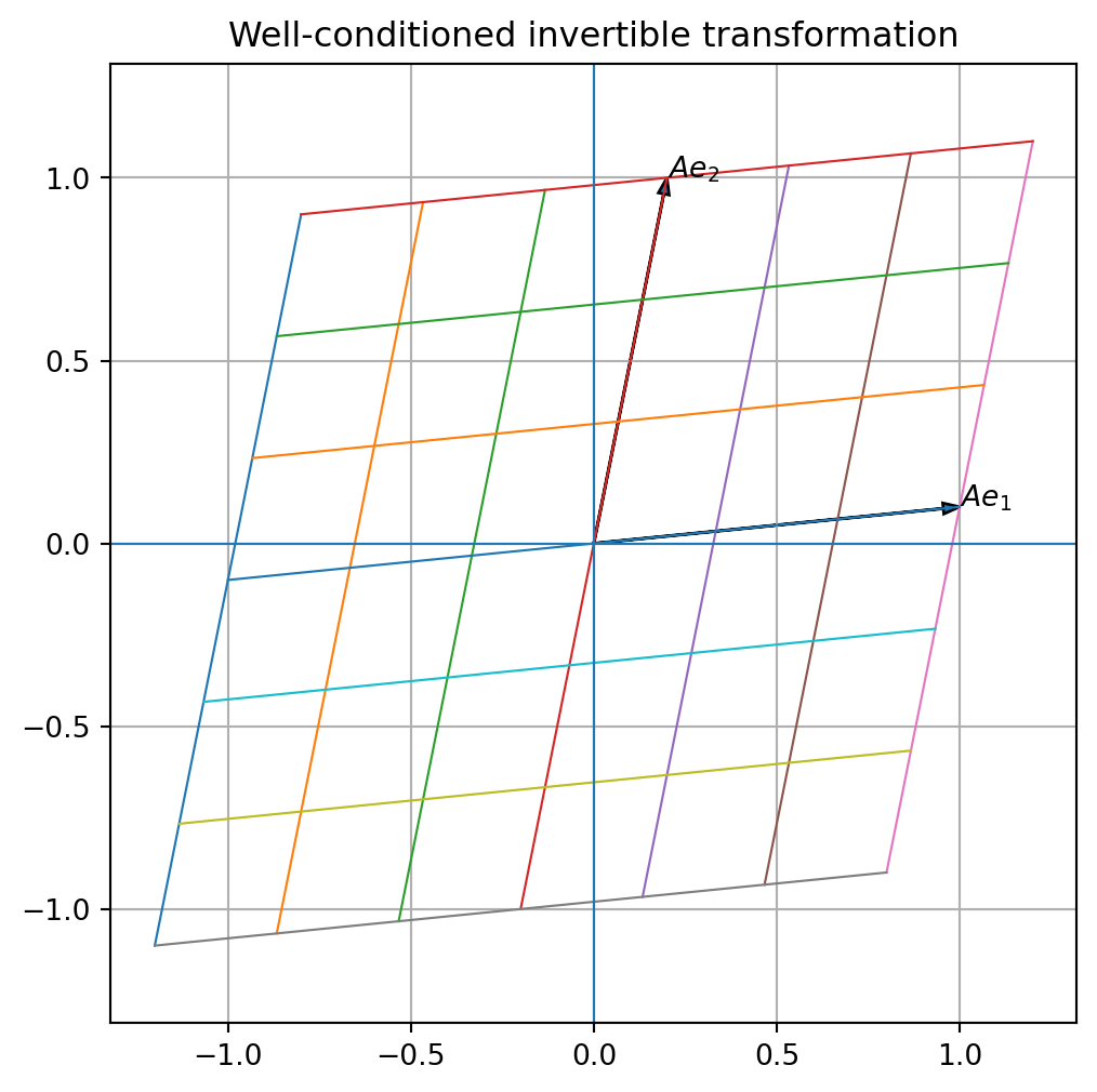
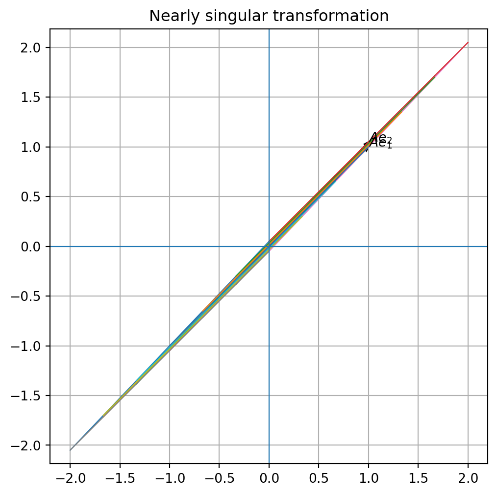
Some matrices are invertible but nearly singular. This means they almost lose information.
For example,
\[
A_\varepsilon=
\begin{bmatrix}
1&1\\
1&1+\varepsilon
\end{bmatrix}.
\]
When \(\varepsilon\) is very small, the two columns are almost the same.
The determinant is
\[
\det(A_\varepsilon)=\varepsilon.
\]
So the matrix is invertible when \(\varepsilon\ne 0\) , but it becomes numerically unstable when \(\varepsilon\) is close to \(0\) .
for eps in [1e-1 , 1e-3 , 1e-6 , 1e-9 ]:= np.array([[1 , 1 ], [1 , 1 + eps]], dtype= float )print (eps, np.linalg.det(Aeps), np.linalg.cond(Aeps))
0.1 0.10000000000000006 42.076233614225764
0.001 0.00099999999999989 4002.000750125414
1e-06 9.999999999177338e-07 4000002.0005977233
1e-09 1.0000000827403716e-09 3999999887.515756
The condition number measures numerical sensitivity. A large condition number means small input errors can cause large output errors.
We will return to this idea when studying least squares and the SVD.
5.23 Common mistakes
Mistake 1: trying to invert a nonsquare matrix
Only square matrices can have inverses in the usual sense.
Rectangular matrices do not have two-sided inverses.
Mistake 2: thinking every square matrix is invertible
Some square matrices are singular. For example,
\[
\begin{bmatrix}
1&2\\
2&4
\end{bmatrix}
\]
does not have an inverse.
Mistake 3: forgetting both inverse equations
The definition requires
\[
A^{-1}A=I
\]
and
\[
AA^{-1}=I.
\]
For square matrices, one condition implies the other, but conceptually the inverse should undo \(A\) from both sides.
Mistake 4: dividing by determinant zero
The \(2\times 2\) inverse formula only works when
\[
ad-bc\ne 0.
\]
Mistake 5: using inverse as the default computational method
In numerical computation, prefer
over
Mistake 6: ignoring near singularity
A matrix can be invertible in exact mathematics but unstable in numerical computation.
5.24 Chapter summary
An \(n\times n\) matrix \(A\) is invertible if there is a matrix \(A^{-1}\) such that
\[
A^{-1}A=AA^{-1}=I_n.
\]
If \(A\) is invertible, then the unique solution of
\[
Ax=b
\]
is
\[
x=A^{-1}b.
\]
For a \(2\times 2\) matrix,
\[
\begin{bmatrix}
a&b\\
c&d
\end{bmatrix}^{-1}
=
\frac{1}{ad-bc}
\begin{bmatrix}
d&-b\\
-c&a
\end{bmatrix},
\]
provided \(ad-bc\ne 0\) .
For general square matrices, compute the inverse by row reducing
\[
[A\mid I]\to [I\mid A^{-1}].
\]
Elementary row operations correspond to multiplying by elementary matrices.
Invertibility is equivalent to:
unique solution for every \(b\) ,
only zero solution to \(Ax=0\) ,
rref\((A)=I\) ,
pivot in every row and column,
independent columns,
columns spanning \(\mathbb{R}^n\) ,
nonzero determinant,
no information loss.
Exercises
A. Inverse definition
Let
\[
A=
\begin{bmatrix}
2&0\\
0&3
\end{bmatrix}.
\]
Find \(A^{-1}\) and verify \(AA^{-1}=I\) .
Let
\[
A=
\begin{bmatrix}
1&0\\
0&-1
\end{bmatrix}.
\]
Show that \(A^{-1}=A\) .
Give a geometric interpretation of the matrix in part 2.
C. Inverses by row reduction
Use Gauss–Jordan elimination to find the inverse, or show that the matrix is not invertible.
\[
\begin{bmatrix}
1&1\\
2&3
\end{bmatrix}
\]
\[
\begin{bmatrix}
1&2\\
2&4
\end{bmatrix}
\]
\[
\begin{bmatrix}
1&1&1\\
1&2&3\\
1&3&6
\end{bmatrix}
\]
\[
\begin{bmatrix}
1&0&1\\
0&1&0\\
2&-1&-1
\end{bmatrix}
\]
D. Solving systems using inverses
For each system, use an inverse to solve.
\[
\begin{bmatrix}
1&2\\
3&4
\end{bmatrix}
x
=
\begin{bmatrix}
5\\
11
\end{bmatrix}
\]
\[
\begin{bmatrix}
2&1\\
1&1
\end{bmatrix}
x
=
\begin{bmatrix}
7\\
4
\end{bmatrix}
\]
\[
\begin{bmatrix}
1&1&1\\
1&2&3\\
1&3&6
\end{bmatrix}
x
=
\begin{bmatrix}
3\\
5\\
8
\end{bmatrix}
\]
E. Elementary matrices
Write the \(3\times 3\) elementary matrix that swaps rows \(1\) and \(3\) .
Write the \(3\times 3\) elementary matrix that multiplies row \(2\) by \(-4\) .
Write the \(3\times 3\) elementary matrix that replaces row \(3\) by row \(3+2\) row \(1\) .
Choose a \(3\times 3\) matrix \(A\) and verify that multiplying by your elementary matrices performs the corresponding row operations.
F. Invertible Matrix Theorem
For each matrix, determine which statements are true:
rref\((A)=I\) ,
\(A\) is invertible,\(Ax=0\) has only the zero solution,the columns of \(A\) span \(\mathbb{R}^n\) ,
the columns of \(A\) are linearly independent.
\[
A=
\begin{bmatrix}
1&2\\
3&4
\end{bmatrix}
\]
\[
A=
\begin{bmatrix}
1&2\\
2&4
\end{bmatrix}
\]
\[
A=
\begin{bmatrix}
1&0&0\\
0&1&0\\
0&0&1
\end{bmatrix}
\]
\[
A=
\begin{bmatrix}
1&1&1\\
1&2&3\\
1&3&6
\end{bmatrix}
\]
G. Geometry
Explain why a matrix whose columns lie on the same line in \(\mathbb{R}^2\) cannot be invertible.
Explain why a matrix that sends a nonzero vector to zero cannot be invertible.
Draw or plot the image of the unit square under
\[
A=
\begin{bmatrix}
1&2\\
2&4
\end{bmatrix}.
\]
What happens?
Draw or plot the image of the unit square under
\[
A=
\begin{bmatrix}
1&1\\
0&1
\end{bmatrix}.
\]
What happens?
H. Python exercises
Use NumPy to compute the inverse of
\[
A=
\begin{bmatrix}
1&1&1\\
1&2&3\\
1&3&6
\end{bmatrix}.
\]
Verify that \(AA^{-1}\) is approximately \(I\) .
Use np.linalg.solve(A,b) to solve
\[
Ax=
\begin{bmatrix}
3\\
5\\
8
\end{bmatrix}.
\]
Compare the answer with np.linalg.inv(A) @ b.
Compute the determinant and condition number of
\[
A_\varepsilon=
\begin{bmatrix}
1&1\\
1&1+\varepsilon
\end{bmatrix}
\]
for \(\varepsilon=10^{-1},10^{-3},10^{-6},10^{-9}\) .
Write a short explanation of what happens as \(\varepsilon\) approaches \(0\) .
AI-age connection
Invertibility means that a linear process loses no information. This idea is important in data compression, numerical stability, optimization, machine learning, and neural networks. In practice, exact invertibility is often less important than approximate invertibility and numerical conditioning. A matrix may be invertible in theory but nearly singular in computation. The condition number, which will reappear later through the SVD, measures how safely a linear transformation can be reversed.