Opening question
A matrix is not only a table of numbers. It is also a rule for moving vectors.
Given a matrix \(A\) , the formula
\[
T(x)=Ax
\]
defines a function from one Euclidean space to another. For example,
\[
A=\begin{bmatrix}2&0\\0&1\end{bmatrix}
\]
stretches vectors horizontally by a factor of \(2\) while leaving vertical components unchanged.
This chapter studies functions that preserve the operations of linear algebra.
A linear transformation is a function that preserves linear combinations.
Learning goals
After studying this chapter, you should be able to:
Define a linear transformation.
Test whether a function is linear.
Understand linear transformations geometrically.
Compute the standard matrix of a linear transformation.
Interpret columns of a matrix as images of standard basis vectors.
Describe the kernel and image of a linear transformation.
Relate kernel and image to nullspace and column space.
Determine whether a linear transformation is one-to-one or onto.
Visualize linear transformations in \(\mathbb{R}^2\) .
Use Python to plot transformed vectors and grids.
10.1 Functions between Euclidean spaces
A function
\[
T:\mathbb{R}^n\to\mathbb{R}^m
\]
assigns to each input vector \(x\in\mathbb{R}^n\) an output vector \(T(x)\in\mathbb{R}^m\) .
For example,
\[
T:\mathbb{R}^2\to\mathbb{R}^2,\qquad
T\left(\begin{bmatrix}x\\y\end{bmatrix}\right)
=
\begin{bmatrix}2x\\y\end{bmatrix}
\]
stretches the \(x\) -coordinate by a factor of \(2\) .
Another example is
\[
S:\mathbb{R}^3\to\mathbb{R}^2,\qquad
S\left(\begin{bmatrix}x\\y\\z\end{bmatrix}\right)
=
\begin{bmatrix}
x+2y-z\\
3x+z
\end{bmatrix}.
\]
This transformation takes vectors in \(\mathbb{R}^3\) and outputs vectors in \(\mathbb{R}^2\) .
10.3 A useful linearity test
A function \(T:\mathbb{R}^n\to\mathbb{R}^m\) is linear if and only if
\[
T(cu+dv)=cT(u)+dT(v)
\]
for all vectors \(u,v\) and all scalars \(c,d\) .
Every linear transformation satisfies
\[
T(0)=0.
\]
Indeed, since \(0=0u\) ,
\[
T(0)=T(0u)=0T(u)=0.
\]
If \(T(0)\ne 0\) , then \(T\) is not linear.
10.6 Examples that are not linear
Translation
\[
T\left(\begin{bmatrix}x\\y\end{bmatrix}\right)
=
\begin{bmatrix}x+1\\y\end{bmatrix}.
\]
Then
\[
T(0)=\begin{bmatrix}1\\0\end{bmatrix}\ne 0.
\]
So \(T\) is not linear.
Squaring
\[
T:\mathbb{R}\to\mathbb{R},\qquad T(x)=x^2.
\]
Then
\[
T(1+1)=4,
\]
but
\[
T(1)+T(1)=2.
\]
So \(T\) is not linear.
Affine maps
A function of the form
\[
T(x)=Ax+b
\]
with \(b\ne 0\) is usually not linear because
\[
T(0)=b\ne 0.
\]
Such functions are called affine transformations.
10.7 The standard matrix
Let \(T:\mathbb{R}^n\to\mathbb{R}^m\) be linear. The standard basis vectors of \(\mathbb{R}^n\) are \(e_1,\ldots,e_n\) .
Every vector can be written as
\[
x=x_1e_1+\cdots+x_ne_n.
\]
By linearity,
\[
T(x)=x_1T(e_1)+\cdots+x_nT(e_n).
\]
Therefore \(T\) is completely determined by what it does to the standard basis vectors.
The standard matrix of \(T:\mathbb{R}^n\to\mathbb{R}^m\) is
\[
A=\begin{bmatrix}T(e_1)&T(e_2)&\cdots&T(e_n)\end{bmatrix}.
\]
Then
\[
T(x)=Ax.
\]
10.8 Example: finding a standard matrix
Suppose
\[
T(e_1)=\begin{bmatrix}2\\1\end{bmatrix},
\qquad
T(e_2)=\begin{bmatrix}-1\\3\end{bmatrix}.
\]
Then
\[
A=
\begin{bmatrix}
2&-1\\
1&3
\end{bmatrix}.
\]
Thus
\[
T\left(\begin{bmatrix}x\\y\end{bmatrix}\right)
=
\begin{bmatrix}
2&-1\\
1&3
\end{bmatrix}
\begin{bmatrix}x\\y\end{bmatrix}
=
\begin{bmatrix}
2x-y\\
x+3y
\end{bmatrix}.
\]
10.9 Columns as images of basis vectors
If
\[
A=\begin{bmatrix}a_1&a_2&\cdots&a_n\end{bmatrix},
\]
then
\[
Ae_1=a_1,\quad Ae_2=a_2,\quad \ldots,\quad Ae_n=a_n.
\]
So the columns of \(A\) tell us where the standard basis vectors go.
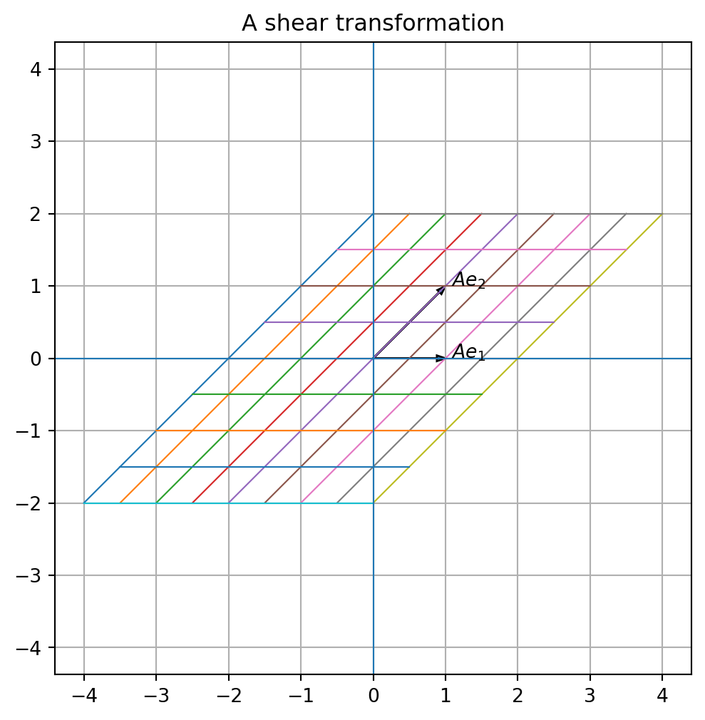
The columns of a matrix are the images of the coordinate axes.
This is one of the most important geometric interpretations of a matrix.
10.12 Kernel
Let \(T:\mathbb{R}^n\to\mathbb{R}^m\) be a linear transformation. The kernel of \(T\) is
\[
\ker(T)=\{x\in\mathbb{R}^n:T(x)=0\}.
\]
If \(T(x)=Ax\) , then
\[
\ker(T)=\operatorname{Null}(A).
\]
The kernel measures information loss. If a nonzero vector is sent to zero, then the transformation collapses a direction.
10.13 Image
Let \(T:\mathbb{R}^n\to\mathbb{R}^m\) be a linear transformation. The image of \(T\) is
\[
\operatorname{im}(T)=\{T(x):x\in\mathbb{R}^n\}.
\]
If \(T(x)=Ax\) , then
\[
\operatorname{im}(T)=\operatorname{Col}(A).
\]
The image is the set of all possible outputs.
The equation
\[
T(x)=b
\]
has a solution exactly when
\[
b\in\operatorname{im}(T).
\]
10.14 Kernel and image are subspaces
If \(T\) is linear, then \(\ker(T)\) is a subspace of the input space and \(\operatorname{im}(T)\) is a subspace of the output space.
For \(T(x)=Ax\) ,
\[
\ker(T)=\operatorname{Null}(A)\subseteq\mathbb{R}^n,
\]
and
\[
\operatorname{im}(T)=\operatorname{Col}(A)\subseteq\mathbb{R}^m.
\]
So the fundamental subspaces of a matrix are also the natural subspaces of a linear transformation.
10.15 One-to-one
A function is one-to-one if different inputs always produce different outputs.
For linear transformations, there is a simple test.
A linear transformation \(T\) is one-to-one if and only if
\[
\ker(T)=\{0\}.
\]
For \(T(x)=Ax\) , this means that the columns of \(A\) are linearly independent.
Equivalently, \(A\) has a pivot in every column.
10.16 Onto
A transformation
\[
T:\mathbb{R}^n\to\mathbb{R}^m
\]
is onto if every vector in \(\mathbb{R}^m\) is an output.
That is, for every \(b\in\mathbb{R}^m\) , there is an \(x\in\mathbb{R}^n\) such that
\[
T(x)=b.
\]
Equivalently,
\[
\operatorname{im}(T)=\mathbb{R}^m.
\]
For \(T(x)=Ax\) , this means that the columns of \(A\) span \(\mathbb{R}^m\) .
Equivalently, \(A\) has a pivot in every row.
10.21 Python: standard matrix from basis images
Suppose
\[
T(e_1)=\begin{bmatrix}2\\1\end{bmatrix},
\qquad
T(e_2)=\begin{bmatrix}-1\\3\end{bmatrix}.
\]
The standard matrix has these vectors as columns.
= np.array([2 , 1 ], dtype= float )= np.array([- 1 , 3 ], dtype= float )= np.column_stack([Te1, Te2])
array([[ 2., -1.],
       [ 1.,  3.]])
For
\[
x=\begin{bmatrix}4\\2\end{bmatrix},
\]
we compute
= np.array([4 , 2 ], dtype= float )@ x
This equals
because
\[
T(4e_1+2e_2)=4T(e_1)+2T(e_2).
\]
10.22 Python: kernel and image
import sympy as sp= sp.Matrix([1 , 0 ],0 , 0 ]
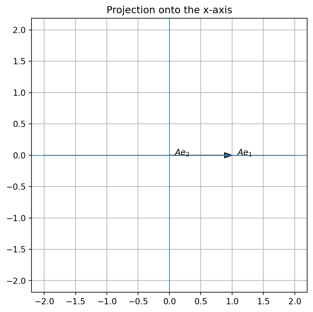
This gives a basis for the kernel of projection onto the \(x\) -axis.
This gives a basis for the image.
For this projection,
\[
\ker(T)=\operatorname{span}\left\{\begin{bmatrix}0\\1\end{bmatrix}\right\},
\]
and
\[
\operatorname{im}(T)=\operatorname{span}\left\{\begin{bmatrix}1\\0\end{bmatrix}\right\}.
\]
10.23 Algorithmic summary
To test whether \(T:\mathbb{R}^n\to\mathbb{R}^m\) is linear:
Check whether \(T(0)=0\) .
Check whether \(T(u+v)=T(u)+T(v)\) .
Check whether \(T(cu)=cT(u)\) .
Equivalently, check whether \(T(cu+dv)=cT(u)+dT(v)\) .
To find the standard matrix of \(T:\mathbb{R}^n\to\mathbb{R}^m\) :
Compute \(T(e_1),T(e_2),\ldots,T(e_n)\) .
Place these vectors as columns:
\[
A=\begin{bmatrix}T(e_1)&T(e_2)&\cdots&T(e_n)\end{bmatrix}.
\]
If \(T(x)=Ax\) , then:
Find \(\ker(T)\) by solving \(Ax=0\) .
Find \(\operatorname{im}(T)\) by finding a basis for \(\operatorname{Col}(A)\) .
For \(T(x)=Ax\) with \(A\) an \(m\times n\) matrix:
\(T\) is one-to-one if \(A\) has a pivot in every column.\(T\) is onto \(\mathbb{R}^m\) if \(A\) has a pivot in every row.
10.24 Common mistakes
Mistake 1: thinking every function with variables is linear
A function is linear only if it preserves addition and scalar multiplication.
Expressions like \(x^2\) , \(xy\) , \(\sin x\) , and \(x+1\) are not linear.
Mistake 2: forgetting \(T(0)=0\)
Every linear transformation sends zero to zero.
If \(T(0)\ne 0\) , the function is not linear.
Mistake 3: confusing kernel and image
The kernel lives in the input space.
The image lives in the output space.
For \(T:\mathbb{R}^n\to\mathbb{R}^m\) ,
\[
\ker(T)\subseteq\mathbb{R}^n,
\]
while
\[
\operatorname{im}(T)\subseteq\mathbb{R}^m.
\]
Mistake 4: putting images of basis vectors as rows
The standard matrix is
\[
A=\begin{bmatrix}T(e_1)&T(e_2)&\cdots&T(e_n)\end{bmatrix}.
\]
The images of standard basis vectors become columns.
10.25 Chapter summary
A linear transformation satisfies
\[
T(u+v)=T(u)+T(v)
\]
and
\[
T(cu)=cT(u).
\]
Equivalently, it preserves linear combinations.
Every matrix transformation \(T(x)=Ax\) is linear.
Every linear transformation \(T:\mathbb{R}^n\to\mathbb{R}^m\) has a standard matrix
\[
A=\begin{bmatrix}T(e_1)&T(e_2)&\cdots&T(e_n)\end{bmatrix}.
\]
The columns of \(A\) are the images of the standard basis vectors.
The kernel is
\[
\ker(T)=\{x:T(x)=0\}.
\]
The image is
\[
\operatorname{im}(T)=\{T(x):x\in\mathbb{R}^n\}.
\]
If \(T(x)=Ax\) , then
\[
\ker(T)=\operatorname{Null}(A),
\]
and
\[
\operatorname{im}(T)=\operatorname{Col}(A).
\]
A linear transformation is one-to-one if its kernel is \(\{0\}\) .
It is onto if its image is the whole output space.
Exercises
A. Testing linearity
Determine whether each function is linear.
\[
T\left(\begin{bmatrix}x\\y\end{bmatrix}\right)
=
\begin{bmatrix}2x\\3y\end{bmatrix}
\]
\[
T\left(\begin{bmatrix}x\\y\end{bmatrix}\right)
=
\begin{bmatrix}x+1\\y\end{bmatrix}
\]
\[
T\left(\begin{bmatrix}x\\y\end{bmatrix}\right)
=
\begin{bmatrix}x+y\\x-y\end{bmatrix}
\]
\[
T(x)=x^2
\]
\[
T\left(\begin{bmatrix}x\\y\\z\end{bmatrix}\right)
=
\begin{bmatrix}x+2y-z\\3x+z\end{bmatrix}
\]
B. Standard matrices
Find the standard matrix of each linear transformation.
\(T:\mathbb{R}^2\to\mathbb{R}^2\) with
\[
T(e_1)=\begin{bmatrix}2\\1\end{bmatrix},
\qquad
T(e_2)=\begin{bmatrix}-1\\3\end{bmatrix}.
\]
\(T:\mathbb{R}^3\to\mathbb{R}^2\) with
\[
T\left(\begin{bmatrix}x\\y\\z\end{bmatrix}\right)
=
\begin{bmatrix}x+2y-z\\3x+z\end{bmatrix}.
\]
Projection onto the \(x\) -axis in \(\mathbb{R}^2\) .
Reflection across the \(y\) -axis in \(\mathbb{R}^2\) .
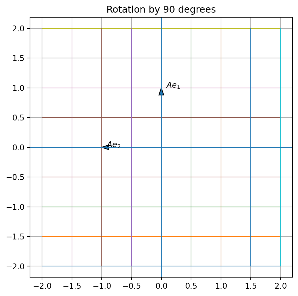
Rotation by \(90^\circ\) counterclockwise in \(\mathbb{R}^2\) .
C. Images of basis vectors
Let
\[
A=
\begin{bmatrix}
1&2&0\\
-1&3&4
\end{bmatrix}.
\]
Compute \(Ae_1\) .
Compute \(Ae_2\) .
Compute \(Ae_3\) .
Explain how these results relate to the columns of \(A\) .
D. Kernel and image
For each matrix \(A\) , find a basis for \(\ker(T)\) and \(\operatorname{im}(T)\) , where \(T(x)=Ax\) .
\[
A=
\begin{bmatrix}
1&0\\
0&0
\end{bmatrix}
\]
\[
A=
\begin{bmatrix}
1&1\\
0&1
\end{bmatrix}
\]
\[
A=
\begin{bmatrix}
1&2&0\\
0&1&1
\end{bmatrix}
\]
\[
A=
\begin{bmatrix}
1&2&3\\
2&4&6
\end{bmatrix}
\]
E. One-to-one and onto
For each transformation \(T(x)=Ax\) , determine whether \(T\) is one-to-one and whether it is onto its codomain.
\[
A=
\begin{bmatrix}1&0\\0&0\end{bmatrix},
\qquad
T:\mathbb{R}^2\to\mathbb{R}^2.
\]
\[
A=
\begin{bmatrix}1&1\\0&1\end{bmatrix},
\qquad
T:\mathbb{R}^2\to\mathbb{R}^2.
\]
\[
A=
\begin{bmatrix}1&2&0\\0&1&1\end{bmatrix},
\qquad
T:\mathbb{R}^3\to\mathbb{R}^2.
\]
\[
A=
\begin{bmatrix}1&0\\0&1\\1&1\end{bmatrix},
\qquad
T:\mathbb{R}^2\to\mathbb{R}^3.
\]
F. Geometry
Plot the image of a square grid under
\[
A=\begin{bmatrix}1&1\\0&1\end{bmatrix}.
\]
Plot the image of a square grid under
\[
A=\begin{bmatrix}1&0\\0&0\end{bmatrix}.
\]
Plot the image of a square grid under
\[
A=\begin{bmatrix}0&-1\\1&0\end{bmatrix}.
\]
Explain which transformations lose information.
G. Python exercises
Write a Python function that plots the image of a grid under a \(2\times 2\) matrix.
Use it for scaling, rotation, reflection, projection, and shear matrices.
Use SymPy to find the kernel and image of
\[
A=
\begin{bmatrix}
1&2&0\\
0&1&1
\end{bmatrix}.
\]
For each square matrix, compute its determinant and relate determinant zero to information loss.
Choose your own \(2\times 2\) matrix and describe the geometric transformation it performs.
H. Reflection
Write a short paragraph answering each question.
Why does linearity mean preserving linear combinations?
Why do the images of the standard basis vectors determine the whole transformation?
How does the kernel describe information loss?
How does the image describe possible outputs?
Why are linear transformations central to data and AI?
AI-age connection
Linear transformations are the basic operations of high-dimensional computation. A neural network layer begins with a linear transformation. A data matrix transforms feature vectors. Dimensionality reduction maps high-dimensional data into lower-dimensional representations. Kernels describe lost information, and images describe possible outputs. Understanding linear transformations gives the geometric foundation for matrix models, optimization, machine learning, and AI.